An exchange-traded fund (ETF) is a type of fund that involves a collection of securities, and often tracks an underlying index
ETFs can invest in any number of industry sectors or use various strategies
ETFs trade on both the primary market and on the secondary markets
Primary Market: Creation and Redemption
ETF shares are created or redeemed in kind, in a shares-for-shares swap
ETF shares are created or redeemed on primary market
Authorized participants(APs) are the large brokers/dealers authorized by the ETF issuer to participate in the creation/redemption process
Creation or redemption happens directly between authorized participants(APs) and the ETF issuer on an over-the-counter basis
APs transfer securities to (for creations) or receive securities from(for redemptions) the issuer, in exchange for ETF shares
Creation basket is the list of securities specific to each ETF
Redemption basket is the basket of securities the AP receives when it redeems the ETF shares
Creation units is the size of transaction between the AP and the ETF manager, usually 50,O0O shares of the ETF
Secondary Market: Trading and Settlement
ETF shares trade intraday on exchanges
AP plays a role of either the broker or the market maker
Settlement
US settlement
Cleared and settled centrally
T+2 settlement
European settlement
Fragmented settlement process
Wider spreads and higher trading costs
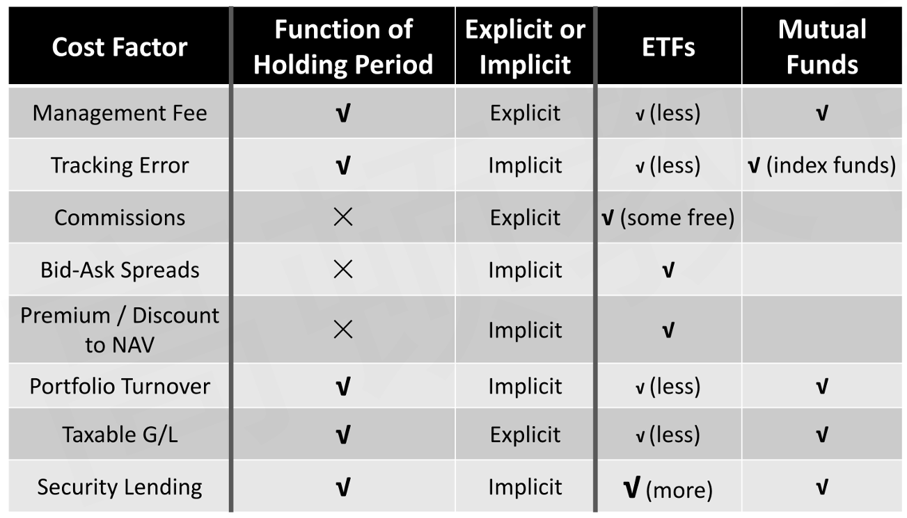
Costs and Risks of ETFs
Trading Costs
Bid-Ask Spreads
Bid-ask spreads represent the market maker's price to take the other side of the ETF transaction
Bid-ask spreads are determined by the following factors:
The market structure
Bid-ask spreads on fixed income relative to equity tend to be wider because the underlying bonds may trade in dealer markets and hedging is more difficult
Different time zones: Spreads on ETFs holding international stocks may be tighter when the underlying security markets are open for trading
Liquidity of the ETFs
More competition among market makers → lower spreads
Higher daily trading volume →lower spreads
Liquidity of the underlying securities
Generally, ETF bid-ask spreads are less than or equal to the combination of the following factors
Creation/redemption fees and other direct trading costs(+, may-)
Such as brokerage and exchange fees
Bid-ask spreads of the underlying securities held in ETFs(+)
Compensation to market maker or liquidity provider(+)
Market makers desired profit spread(+)
Subject to competitive forces
Discount related to receiving an offsetting ETF order (-)
Premiums and Discounts to NAV
ETF premiums and discounts refer to the difference between the exchange price of the ETF and the fund's calculated NAV
iNAV, or "indicated" NAV, are intraday "fair value" estimates of an ETF share based on its creation basket composition
An ETF is said to be trading at a premium when its share price is higher than iNAV or NAV, and at a discount if its price is lower than iNAV or NAV
End-of-day ETF premium or discount (%) = (ETF price - NAV per share) / NAV per share
Intraday ETF premium or discount (%) = (ETF price - iNAVper share) / iNAV per share
Premiums/discounts are driven by a number of factors
Timing differences: NAVs are based on underlying securities' last traded prices, which may be observed at a time lag to the ETFs' price
ETF and the underlying security trade on different exchanges
Some underlying securities trade in dealer market
Stable pricing
ETFs may be more liquid and more reflective of current information
Or, infrequently traded ETFs
Tracking Error
Index Tracking
For index-tracking ETFs,ETF managers attempt to deliver performance that tracks the fund's benchmark as closely as possible
Index-tracking ETFs dominate in the ETF markets
Index tracking is evaluated using the one-day or periodic difference in returns between the fund (as measured by its NAV) and its underlying index
Tracking Error
Tracking error is defined as the standard deviation of differences in performance between the index and the fund tracking the index
Tracking error does not reveal the extent to which the fund is under or over performing its index or anything about the distribution of errors
Sources of Tracking Error
Fees and expenses
Index calculation generally assumes that trading is frictionless and occurs at the closing price
A fund's operating fees and expenses reduce the fund's return relative to the index
Representative sampling and optimization
For funds tracking index exposure to small or illiquid markets,owning every index constituent can be difficult and costly
Depositary receipts and other ETFs
When local market shares are illiquid, ETF managers may choose to hold depositary receipts instead of local constituent shares
Although the economic exposure is equivalent, differences in trading hours and security prices create discrepancies between portfolio and index values, such as American depositary receipts (ADRs),global depositary receipts(GDRs)
Index changes
The more volatile the market, the wider the bid-offer spreads and range of traded prices
Fund accounting practices
Differences in valuation practices between the fund and its index can create discrepancies that magnify daily tracking differences
Regulatory and tax requirements
Asset manager operations Security lending or foreign dividend recapture income is not accounted for in the index calculation
Tax Issues
Tax Fairness
Mutual funds
When an investor sells, the fund must sell portfolio securities to raise cash to pay the investor
Any securities sold at a profit incur a capital gains charge, which is distributed to remaining shareholders
ETFs
An investor sells ETF shares to another investor in the secondary market do not require the fund to trade out of its underlying positions
If an AP redeems ETF shares, this redemption occurs in kind and is not a taxable event
Tax Efficiency
Tax lot management allows portfolio managers to limit the unrealized gains in a portfolio
When an authorized participant submits shares of an ETF for redemption, the ETF manager can choose which underlying share lots to deliver in the redemption basket
By choosing shares with the largest unrealized capital gains (those acquired at the lowest cost basis), ETF managers can use the in-kind redemption process to reduce potential capital gains in the fund
Other Distributions
Other events, such as security dividend distributions, can trigger tax liabilities for investors
In most markets,ETFs distribute their accumulated dividends
In some jurisdictions (eg. Europe), ETFs may have share classes that accumulate and automatically reinvest dividends into the fund
Other Costs and Risks Of Owning ETFS
Expense Ratios
ETFs generally charge lower fees than mutual funds
Do not have to keep track of individual investor accounts
Do not bear the costs of communicating directly with individual investors
Do not require the security and macroeconomic research carried out by active managers
The actual costs to manage an ETF vary
Portfolio complexity
Issuer size
Competitive landscape
Settlement risk
Some ETFs may use over-the-counter (OTC) derivatives, such as swaps, to gain market exposure has settlement risk
Security lending
ETF issuers lend their underlying securities to short sellers,earning additional income for the fund's investors
Securities lent are generally overcollateralized, so that the risk from counterparty default is low
Fund closures
Regulation/Competition /Corporate actions
Soft closures: Creation halts / Change in investment strategy
Investor related risk
Investors do not fully understand the underlying exposure
Leveraged and inverse ETFs
ETFs in Portfolio Management
Advantages
Portfolio liquidity management
ETFs can be used to invest excess cash balances quickly(known as cash equitization), thereby minimizing potential cash drag
Managers may also use ETFs to transact small cash flows originating from dividends, income, or shareholder activity
Transacting the ETF may incur lower trading costs and be easier operationally than liquidating underlying securities or requesting funds from an external manager
Portfolio rebalancing
Using liquid ETFs allows the portfolio remains fully invested according to its target weights
Portfolio completion strategies
If external managers are collectively underweighting or overweighting an industry or segment, ETFs can be used to adjust exposure up or down to the desired level
Transition management
Transition management refers to the process of hiring and firing managers, or making changes to allocations with existing managers,while trying to keep target allocations in place
Asset owners can use ETFs to maintain desired market or asset class exposure in the absence of having an external manager in place
Asset class exposure management
Core exposure to an asset class or sub-asset class
Tactical strategies
Active and factor investing
Factor(smart beta) ETFs
Risk management
Alternatively weighted ETFs
Discretionary active ETFs
Dynamic asset allocation and multi-asset strategies
Drawbacks
For very large asset owners, there are potential drawbacks to using ETFs for portfolio management
Given the asset owner size, they may be able to negotiate lower fees for a dedicated separately managed account(SMA) or find lower-cost commingled trust accounts that offer lower fees for large investors
An SMA can be customized to the investment goals and needs of the investor
Many regulators require large ETF holdings to be disclosed to the public
This can detract from the flexibility in managing the ETF position and increase the cost of shifting investment holdings
Multifactor Models
Arbitrage Pricing Theory
Arbitrage Pricing Model
APT introduced a framework that explains the expected return of a portfolio in equilibrium as a linear function of the risk of the portfolio with respect to a set of factors capturing systematic risk
E(R_P)=R_f+\sum\beta_{P,i}\lambda_i
\beta_{P,i} is the sensitivity of the portfolio to factor i
\lambda_i is the expected risk premium for risk factor i, also called factor risk premium
Pure Factor Portfolio
Pure factor portfolio is a portfolio with sensitivity of 1 to factor i and sensitivity of 0 to all other factors
\lambda_i from APT model is also the risk premium for a pure factor portfolio for factor i
Assumptions of APT
A factor model describes asset returns
There are many assets, so investors can form well-diversified portfolios that eliminate asset-specific risk
No arbitrage opportunities exist among well-diversified portfolios
The parameters of the APT equation are the risk-free rate and the factor risk-premiums
The factor sensitivities are specific to individual investments
APT model provides an expression for the expected return of asset assuming that financial markets are in equilibrium
APT model makes less assumptions than CAPM and does not identify the specific risk factors as well as the number of risk factors
CAPM can be regarded as a special case of APT model with only one risk factor (market risk factor)
Arbitrage Opportunity
An opportunity to conduct an arbitrage: earn an expected positive net profit without risk and with no net investment of money
If two portfolios with identical risk factors and factor sensitivities have different return, there is an arbitrage opportunity
Multifactor Models
Structure of Multifactor Models
Macroeconomic Factor Model R_i=E(R_i)+\beta_{i,1}F_1+\cdots+\beta_{i,k}F_k+\varepsilon_i
R_i is the return to asset i, and e(R_i) is the expected return to asset i
F_k is the surprise in in macroeconomic variables, like GDP, interest rate,inflation, credit spreads, etc.
Surprise is the difference between realized value and predicted value
\beta_{i,k} is the sensitivity of the return on asset i to a surprise in factor k
If we have adequately represented the sources of common risk (the factors),then ε; must represent an asset-specific risk
For a stock, it might represent the return from an unanticipated company-specific event
Fundamental Factor Model R_i=a_i+\beta_{i,1}F_1+\cdots+\beta_{i,k}F_k+\varepsilon_i
R_i is the return to asset i
F_k is the return associated with the factor k, which are asset attributes that are important in explaining cross-sectional differences in stock prices, like P/B ratio, P/E ratio, earning growth rate, etc.
\beta_{i,k} is the standardized beta of attributes k of the asset i
Statistical Factor Model
In a statistical factor model, statistical methods are applied to historical returns of a group of securities to extract factors that can explain the observed returns of securities in the group
Major weakness: In contrast to macroeconomic models and fundamental models, factors from statistical factor models are difficult to interpret economically
Major advantage: Statistical factor models make minimal assumptions
Two major types of statistical factor models are factor analysis models and principal components models
In factor analysis models, the factors are the portfolios of securities that best explain (reproduce) historical return covariances
In principal components models, the factors are portfolios of securities that best explain (reproduce) the historical return variances
Comparison between Models
Interpretation of intercept term
Macroeconomic factor model: the asset's expected return based on market expectations(e. g.APT)
Fundamental factor model: regression intercept
Interpretation of factors
Macroeconomic factor model: surprises in the macroeconomic variables
Fundamental factor model: return associated with asset attributes
Return from factor tilts is earned by taking different factor exposures compared to the benchmark, by overweight or underweight relative to the benchmark factor sensitivities
Security Selection Return
Return form security selection is earned by allocating different weights to securities compared to the benchmark
It reflects the ability to overweight securities that outperform the benchmark or underweight securities that underperform the benchmark
Risk Attribution
Active risk is the standard deviation of active returns
The active risk of a portfolio can be separated to two parts
Active risk squared = Active factor risk + Active specific risk
Active factor risk is the contribution to active risk squared resulting from the portfolios different than benchmark exposures relative to factors specified in the risk model
Active specific risk or security selection risk is the contribution to active risk squared resulting from the portfolios active weights on individual assets as those weights interact with assets' residual risk
Portfolio Construction and Decisions
Portfolio Construction
Multifactor models permit the portfolio manager to make focused bets or to control portfolio risk relative to the benchmark's risk
In evaluating portfolios, analysts use multifactor models to understand the sources of managers' returns and assess the risks assumed relative to the manager's benchmark
Passive management: Analysts can use multifactor models to match an index fund's factor exposures to the factor exposures of the index tracked
Active management: Analysts can use multifactor models in predicting excess risk adjusted return or relative return (the return on one asset or asset class relative to that of another) as part of a variety of active investment strategies
Strategic Portfolio Decisions
By introducing more risk factors, multifactor models enable investor gain from taking more or less exposures to risks that they have a comparative advantage / disadvantage
By considering multiple sources of systematic risk, multifactor models allow investors to achieve better diversified and possibly more efficient portfolios
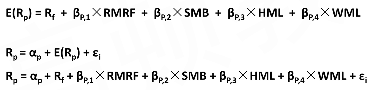
Carhart Model
The Carhart four-factor model can be viewed as an extension of CAPM,and also is an extension of the three-factor model developed by Fama and French
R_P and R_f are the return on the portfolio and the risk-free rate of return, respectively
\alpha_P is the return in excess of that expected given the portfolio's level of systematic risk (assuming the four factors capture all systematic risk)
\beta_P is the sensitivity of the portfolio to the given factor
\varepsilon_i is an error term that represents the portion of the return to the portfolio not explained by the model
RMRF is the return on a value-weighted equity index in excess of the one-monthT-bill rate
SMB represents "small minus big", a size factor,is the average return on small-cap portfolios minus the average return on large-cap portfolios
HML represents "high minus low", a value factor,is the average return on high book-to-market portfolios minus the average return on low book-to-market portfolios
WML represents "winners minus losers", a momentum factor,is the return on a portfolio of the prior winners minus the return on a portfolio of the prior losers
Measuring and Managing Market Risk
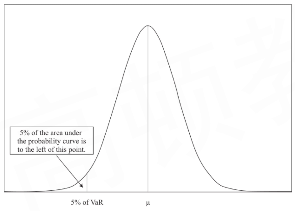
Value at Risk
Definition of VaR
Value at risk is an estimate of the maximum (or minimum) expected loss at a specified level of probability over a specified time period
It associated with a given probability
It has a time element and cannot be compared directly unless they share the same time interval
VaR is usually expressed either as a percentage(% VaR) or in units of currency($ VaR)
In practical, it is more common to state VaR using a confidence level
A 1% VaR would be expected to show greater risk than a 5% VaR
The VaR time period should relate to the nature of the situation
A traditional stock and bond portfolio would likely focus on a longer monthly or quarterly VaR, while a highly leveraged derivatives portfolio might focus on a shorter daily VaR
The left-tail should be examined
The left side of a traditional probability distribution displays the low or negative returns, which is what VaR measures at some probability
Methods to Estimate VaR
Parametric Method
Assume that asset returns conform to a normal distribution
VaR for a portfolio, which contains asset A and asset B(E(R_A)=E(R_B)=0)
\begin{align}
&VaR_{\%}=\sqrt{w_A^2VaR_{A,\%}^2+w_B^2VaR_{B,\%}^2+2\rho_{A,B}w_Aw_BVaR_{A,\%}VaR_{B,\%}}
\\
&VaR_{\$}=\sqrt{VaR_{A,\$}^2+VaR_{B,\$}^2+2\rho_{A,B}VaR_{A,\$}VaR_{B,\$}}
\end{align}
Square Root Rule(E(R)=0) VaR_{\text{T day}}=VaR_{\text{1 day}}\times\sqrt T
Advantage
Simple and straightforward
Disadvantage
Its estimates will only be as good as the estimate of the parameter (mean, variance, covariance)
The usefulness is limited when normality assumption is not reasonable
E.g. when the investment portfolio contains options
Many assets exhibit leptokurtosis
Historical Simulation Method
Given the historical returns and sort the results from largest loss to greatest gain, find out VaR
Imagine that the returns from a portfolio over the past 300 days have been computed and ranked in order from best to worst
We can say that on only 5% of the days was the return worse than or equal to the return placed in the 286th position
Hence the one-day VAR estimate will be the return placed 286th in the list (multiplied by the current portfolio value, if we want the absolute $ VaR)
Advantage
No normality or any other distribution assumption
Available to estimate the VaR for portfolio with options Based on what actually happened, so it cannot be dismissed as introducing impossible outcomes
Based on what actually happened, so it cannot be dismissed as introducing impossible outcomes
Disadvantage
No certainty that a historical event will re-occur, or that it would occur in the same manner or with the same likelihood as represented by the historical data
If data in the lookback period is more volatile, VaR will be over-estimate
If data in the lookback period is less volatile, VaR will be under-estimate
Both parametric and historical simulation methods has a shortage that all observations are weighted equally
Improvement: giving more weight to more recent observations and less weight to more distant observations
Monte Carlo Simulation Method
The user develops his own assumptions about the statistical characteristics of the distribution and uses those characteristics to generate random outcomes that represent hypothetical returns to a portfolio
A computer program simulates the changes in value of the portfolio through time and run repeatedly to produce a set of possible end-of-horizon values
This modelled distribution of portfolio values can then be used to estimate the VaR
Advantage
It can accommodate virtually any distribution
It can accurately incorporating the effects of option positions or bond positions with embedded options
More flexible than the other two methodologies
Disadvantage
Assumptions of inputs are critical for accuracy of estimates
Complex: great deal of computer time and calculations
Extensions of VaR
Advantages of VaR
Simple concept
Easily communicated concept
Provides a basis for risk comparison
Facilitates capital allocation decisions
Can be used for performance evaluation
Reliability can be verified
Widely accepted by regulators
Disadvantages of VaR
It dose not tell us what happened below the VaR and may underestimate the frequency of extreme events
Subjectivity that various methods can generate different values
Oversimplification that it is a single measure that gives limited information
Accuracy of VaR can only be determined after the fact (back testing)
It can underestimate size and frequency of the worst losses if assumptions and models are incorrect
Sensitivity to correlation risk
VaR for individual positions does not easily sum up to a portfolio VaR
Disregard of right-tail events
Failure to take into account liquidity
Misunderstanding the meaning of VaR
Vulnerability to trending or volatility regimes
Conditional VaR(CVaR)
The average loss that would be incurred if the VaR cutoff is exceeded
Also named "expected tail loss"or "expected shortfall"
Incremental VaR(IVaR)
The difference in VaR between the "before" and "after" VaR if a position size is changed relative to the remaining positions
Marginal VaR(MVaR)
The change in VaR for a small change in a given portfolio holding
MVaR is the slope of VaR-weight curve for a security in the portfolio
Approximately, MVaR is the change in VaR for a $1 or 1% change in the position for a security in the portfolio
Relative VaR
A measure of the degree to which the performance of a given investment portfolio might deviate from its benchmark
Also named ex ante tracking error
Other Risk Measures
Sensitivity Risk Measures
Examine how portfolio value responds to a small change in a single risk factor
Equity exposure measures: Beta
Fixed-income exposure measures: duration and convexity
Options risk measures: Delta, Gamma, Vega, etc.
Advantages
Sensitivity risk measures can inform a portfolio manager about a portfolio's exposure to various risk factors to facilitate risk management
If too much/less risk exposure to a risk factor, the manager can modify the exposure accordingly
Limitations
Sensitivity risk measures can only be used to estimate the effects of small changes in risk factors
Even combination of first-order and second-order effects only provide approximation for large changes in risk factors
Two portfolios with same sensitivity risk measures can have different risk due to different volatility of risk factors
Two fixed income portfolios with same duration but different yield volatilities.
Scenario Risk Measures
Hypothetical scenario approach uses a set of hypothetical change in risk factors, not just those that have happened in the past
Stress tests examine the impact on portfolio of a scenario of extreme changes of risk factors
Stress tests can determine the size of change on a certain risk factor that could compromise the sustainability of the investment
Scenario analysis can be regarded as the final step in the risk management process, after performing sensitivity analysis
Scenario analysis can provide additional information on a portfolio's vulnerability to changes of risk factors or the correlations between risk factors.
Advantages
Scenario risk measures can focus on extreme outcomes, but not bound by either recent historical events or assumptions about parameters or probability distributions
Allowing liquidity to be taken into consideration
Scenario analysis is an open-ended exercise that could look at positive or negative events, although its most common application is to assess the negative outcomes
Stress tests intentionally focus on extreme negative events
Limitations
Sensitivity risk measures can only be used to estimate the effects of small changes in risk factors
Even combination of first-order and second-order effects only provide approximation for large changes in risk factors
Two portfolios with same sensitivity risk measures can have different risk due to different volatility of risk factors
Two fixed income portfolios with same duration but different yield volatilities.
Choices of Risk Measures
The choices of risk measures by an organization is mainly decided by
Types of risks it faces
Regulation that govern it
Whether it uses leverage
Banks
Banks need to balance a number of competing aspects of risk to manage their business and meet the expectations of equity investors/analysts,bond investors, credit rating agencies, depositors, and regulatory entities
The typical risk measures used by banks
Liquidity gap
Economic capital
VaR
Sensitivity measures
Scenario analysis and stress tests
Leverage risk measures
Asset Managers
Traditional asset managers focus on relative risk measures
The typical risk measures used by traditional asset managers
Position limits
Sensitivity measures
Scenario analysis
Active share
VaR
Liquidity
Redemption risk
Tracking error VaR
Hedge funds managers focus on absolute return
The typical risk measures used by hedge asset managers
Sensitivity measures
Leverage
VaR
Scenario analysis
Drawdown
Pension Funds
The risk management goal for defined benefit pension funds is to be sufficiently funded to make future payments to pensioners
The typical risk measures used by pension funds
Sensitivity measures
Surplus at risk
Interest rate and curve risk
Insurers
The typical risk measures used by property and casualty insurers
sensitivities and exposures
Economic capital
VaR
Scenario analysis
The typical risk measures used by life Insurers
Sensitivities
asset and liability matching
scenario analysis
Managing Market Risk
Risk budgeting: determining the overall risk appetite, and then allocated to sub-activities or business units
Capital allocation is the practice of placing limits on each of a company's activities in order to ensure that the areas in which it expects the greatest reward and has the greatest expertise are given the resources needed to accomplish their goals
Risk measures must be introduced when limit the overall risk and allocate risk across the activities or business units by risk budgeting
Position limits
The maximum currency amount or percentage of portfolio value allowed for specific asset or asset class
Scenario limits
Limits on expected loss for a given scenario
Stop-loss limits
Require an investment position to be reduced or closed out when losses exceed a given amount over a specified time period
Backtesting and Simulation
Objectives and Steps in Backtesting an Investment Strategy
Backtesting approximates the real-life investment process by using historical data to assess whether a strategy would have produced desirable results
Backtesting can be employed as a rejection or acceptance criterion for a strategy
Steps in backtesting an investment strategy
Strategy design
Specify investment hypothesis and goal(s)
Determine investment rules, process and key parameters
Historicalinvestment simulation
Form and rebalance investment portfolios for each period according to the rules
Analysis of backtesting output
Calculate portfolio performance statistics
Reported Metrics and Visuals
Metrics
Average return
Volatility
Downside risk(e.g.VaR, CVaR, and maximum drawdown)
Sharpe ratio, Sortino ratio
Visuals
An intuitive way of summarizing many data points
Although backtesting fits quantitative and systematic investment styles more naturally, it has also been heavily used by fundamental managers
Problems in Backtesting an Investment Strategy
Survivorship bias refers to deriving conclusions from data that reflects only those entities that have survived to that date
Point-in-time data allows analysts to use the most complete data for any given prior time period
Look-ahead bias is created by using information that was unknown or unavailable during the historical periods over which the backtest is conducted
Survivorship bias is actually a type of look-ahead bias
Data snooping is a type of selection bias, and it occurs when an analyst selects data or performs analyses until a significant result is found
Otherwise known as "p-hacking"
Historical Scenario Analysis
Rather than simply acknowledging or even ignoring structural breaks evident in backtesting results, an analyst should pay careful attention to different structural regimes and impacts to a strategy during regime changes
Historical scenario analysis is a type of backtesting that explores the performance and risk of an investment strategy in different structural regimes and at structural breaks
Two common examples of regime changes are from economic expansions to recessions and from low-volatility to high-volatility environments
Historical Simulation
Historical simulation constructs results by selecting returns at random from many different historical periods without regard to time-ordering
Historical simulation assumes that past asset returns provide sufficient guidance about future asset returns
Historical simulation assumes the data are stationary
Sampling from the historical returns can be with replacement or without replacement
Sampling with replacement, also known as bootstrapping, is more common, because the number of simulations needed is often larger than the size of the historical dataset
Monte Carlo Simulation
Each key variable is assigned a statistical distribution, and observations are drawn at random from the distribution
The distribution should reasonably describe the key empirical patterns of the underlying data
The correlations between multiple key decision variables should be accounted for, and it is necessary to specify a multivariate distribution rather than modeling each factor or asset on a standalone basis
Flexible, but complex
Sensitivity Analysis
Sensitivity analysis is a technique for exploring how a target variable and risk profiles are affected by changes in input variables
It can be implemented to help managers further understand the potential risks and returns of their investment strategies
Economics and Investment Markets
Framework for Analysis
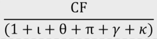
Discounted Cash Flow Model
The value of any asset can be calculated as the present value of its expected cash flows
If a economic factor affects an asset's market value, it must affect one or more of the following
The timing and/or amount of the expected cash flows
One or more of the discount rate components
Default-free interest rate
Expected inflation
Risk premiums
Role of Expectation
Asset values depend on the expectation of future cash flows,which is based on current information that may be relevant to forecasting future cash flows
Asset values may need to be adjusted due to the fact that the unanticipated information arise, as the current asset values only reflect the expected information
Discount Rate
Real Default-Free Rate of Return
The choice to invest today involves the opportunity cost of not consuming today
The tradeoff is measured by the marginal utility of consumption in the future relative to the marginal utility of consumption today
The marginal utility of consumption of investors diminishes as their wealth increases because they have already satisfied fundamental needs
Inter-Temporal Rate of Substitution(ITRS)
Inter-temporal rate of substitution is the ratio of the marginal utility of consuming 1 unit in the future (U_t) to the marginal utility of consuming 1 unit today (U_0), denoted by m_t=U_t/U_0
m_t is always less than 1 because investor always prefer current consumption over future consumption
The inter-temporal rate of substitution is lower at good state of the economy
Discount Rate on Real Default-Free Bond
Assuming a zero coupon, inflation-indexed, risk-free bond with par value of $1, its price today (P_0) should be m_t
If the investment horizon for TIPs is one year, and the payoff then is $1, then the return this bond is R_{real}=\frac{1-P_0}{P_0}=\frac{1}{m_1}-1
The one-period real risk-free rate is inversely related to the inter-temporal rate of substitution
Real risk free rate is positively related to GDP growth rate
Real risk free rate is also positively with the volatility of the growth rate due to higher "risk premium"
Inflation Premium
Short-Term Nominal Interest Rate
Treasury bills (T-bills) are very short-dated nominal zero-coupon government bonds
The yield is short-term nominal default-free interest rate, which s influenced by
The inflation environment and inflation expectations over time. It will also vary with the level of real economic growth and with the expected volatility of that growth Real economic activity, which is influenced by the saving and investment decisions of households
The central bank's policy rate, which should fluctuate around neutral policy
Taylor Rule
Taylor rule provides the targeted short-term rate to balance the risks of inflation and recession
Used as a prescriptive tool to show what target rate will achieve the desired growth
As a forecasting tool to predict actions of the central bank
R=R_{\text{netural}}+\theta+\frac{1}{2}\times(\theta-\theta^\ast)+\frac{1}{2}\times(Y-Y^\ast) R is the central bank policy rate implied by the Taylor rule R_{\text{netural}} is the neutral real policy interest rate \theta is the current inflation rate and \theta^\ast is the target inflation rate Y is the growth of actual real GDP and Y^\ast is the growth of target real GDP
Short-Term vs. Long-Term
Unless the investment horizon is very short, investors are unlikely to be very confident in their ability to forecast inflation accurately
Because we generally assume that investors are risk averse and thus need to be compensated for taking on risk as well as seeking compensation for expected inflation, they will also seek compensation for taking on the uncertainty related to future inflation
For long-term nominal risk-free interest rate, the following effects of inflation should be considered
Premium for expected inflation(\theta)
Risk premium for uncertainty about actual inflation (\pi)
Break-Even Inflation Rate
Break-even inflation rate (BEI) is the yield difference between a non-inflation-indexed risk-free bond and the inflation-indexed risk-free bond with the same maturity
The BEI captures the effects of inflation on yield
BEI=\theta+\pi
Slope of Yield Curve
During the recession, the slope of yield curve will increase
Central bank tends to lower the policy rate
Investors expect higher future GDP growth and higher long-term rates as economic growth recovers
During the recession, short-term bonds generally perform better than long-term bonds Later stages of expansion often have negatively sloped (inverted) yield curve
Typically, high inflation and high short-term interest rate
Low long-term rates due to expectations of decreasing inflation and GDP growth
During the expansion, long-term bonds generally perform better than short-term bonds
Credit Premium
Credit spread(\gamma) is the yield difference between a credit risky bond and a default-free bond with same maturity
It reflects the risk premium for credit risk
Credit spreads tends to narrow in times of robust economic growth, when defaults are less common
Credit risky (lower-rated) bonds will perform better than default-free (higher-rated) bonds
Credit spreads tend to rise in times of economic weakness, as the probability of default rises
Default-free (higher-rated) bonds will perform better than credit risky (lower-rated) bonds
Industry Sector and Company Specific Factors
Some industrial sectors are more sensitive to the business cycle than others
During economic downturn, the credit spread on the consumer cyclical sector rises more dramatically than it do for corporate bonds in the consumer non-cyclical sector
Issuers that are profitable, have low debt interest payments, and that are not heavily reliant on debt financing will tend to have a high credit rating
Sovereign Credit Risk
The credit risk embodied in bonds issued by governments in emerging markets is normally expressed by comparing the yields on these bonds with the yields on bonds with comparable maturity issued by the US
The basic reason for the increase in the credit risk premium was a reassessment by investors of these sovereign issuers ability to pay and the likelihood that they might default
Equity Risk Premium
Yield for equity: \iota +\pi+\theta+\lambda
\lambda is the equity risk premium
The equity risk premium is typically higher than credit risk premium because equity is more risky than debt (\lambda\gt\gamma)
\kappa is essentially the equity risk premium relative to credit risky bonds
Consumption-Hedging Property
Consumption-hedging property describe the feature that may provide high payoff during economic downturns
Assets with more consumption-hedging property will be more highly valued and have less risk premium
The consumption-hedging properties for equities are poor
Sharp falls in equity prices are associated with recessions
Equities are with "bad" consumption hedge, and we would thus expect the equity risk premium to be positive and investors will demand a higher equity risk premium
Valuation Multiples
Valuation multiples are positively related to expected earning growth rate, and negatively related to required rate of return
Booming (recession) economy tends to lead to a rise (decline) of the earning growth expectations
Earning growth rate tend to be relatively stable throughout the business cycle for defensive or non-cyclical industries
Investment Strategy
A value strategy performs well during recession, while growth strategy performs well during expansion
Growth stocks
Strong earnings growth
High P/E and low dividend yield
Have low (or no) positive earnings
Value stocks
Operates in more mature markets with a lower earnings growth
Low P/E and high dividend yield
Capitalization
Small-cap stocks tend to underperform large-cap stocks in difficult economic conditions.
Small-cap companies will tend to have less diversified businesses
Small-cap companies have more difficulty in raising financing particularly during recessions, and will thus be less able to weather an economic storm
Higher risk premium demanded by investors to invest in small-cap stocks relative to large-cap stock due to higher volatility
Rotation Strategies During economic expansion
Rotating into growth stocks when they are expected to outperform value stocks
Rotating into small-cap stocks when they are expected to outperform large-cap stocks
Rotating into cyclical stocks when they are expected to outperform countercyclical stocks
liquidity Premium
Commercial real estate investment have the following characteristics
Bond-like characteristics: steady rental income stream, like cash flows of bonds
Equity-like characteristics: uncertain value of the property at the end of the lease term
Iliquidity
Liquidity Premium
Most of the asset classes are liquid relative to an investment in commercial property
Investors will demand a high risk premium for commercial real estate investment due to weak consumption-hedging properties
Investors will demand a liquidity risk premium \phi
Commercial property value tend to decline in bad times
Active Portfolio Management
Value Added by Active Management
Definition of Value Added
The value added or active return is defined as the difference between the return on the manager's portfolio and the return on a benchmark portfolio
R_A=R_P-R_B
Active Weights
R_A=R_P-R_B=\sum\Delta w_iR_i=\sum\Delta w_iR_{A,i}
\Delta w_i=w_{P,i}-w_{B,i} represents active weights
R_{A,i}=R_i-R_B represents active security return
Individual assets can be overweighed (have positive active weights'or underweighted (have negative active weights), but the complete set of active weights sums to zero
Decomposition of Value Added
For portfolio with multiple asset classes, active return can be decomposed to two sources
R_A=\sum(w_i^P-w_i^B)R_i^B+\sum w_i^P(R_i^P-R_i^B)
Active asset allocation: active weights of asset classes against benchmark portfolio
Security selection: active weights of security within asset classes
Information Ratio
Sharpe Ratio and Information Ratio
Sharpe Ratio
SR_P=\frac{R_P-r_f}{\sigma_P}
Sharpe ratio measures the total risk-adjusted value added, and calculated as excess return per unit of risk
Sharpe ratio is unaffected by the addition of cash or leverage,because excess return and risk will change proportionally
Sharpe ratio is affected by the change of aggressive active weight
Information Ratio
IR_p=\frac{R_P-R_B}{\sigma_{(R_P-R_B)}}
Information ratio measure the relative risk-adjusted value added,and calculated as active returns per unit of active risk
Ex-anti IR is based on expected return
Ex-post IR is based on realized return
Key Conclusions about Information Ratio
Information ratio is unaffected by taking positions in benchmark portfolio
Information ratio is unaffected by the aggressiveness active weight
Information ratio is affected by the addition of cash or use of leverage
Construct Optimal Portfolio
SR and IR
The optimal portfolio will be constructed if SR_P^2=SR_B^2+IR^2
For any given asset class, an investor should choose the manager with the highest expected skill as measured by the information ratio
Because investing with the highest IR manager will produce the highest SR for the investor's portfolio
Optimal Amount of Active Risk
\sigma_{(R_P-R_B)}^\ast=\frac{IR}{SR_B}\times\sigma_{R_B}
For unconstrained portfolios, the level of active risk that leads to the optimal result
The Fundamental Law
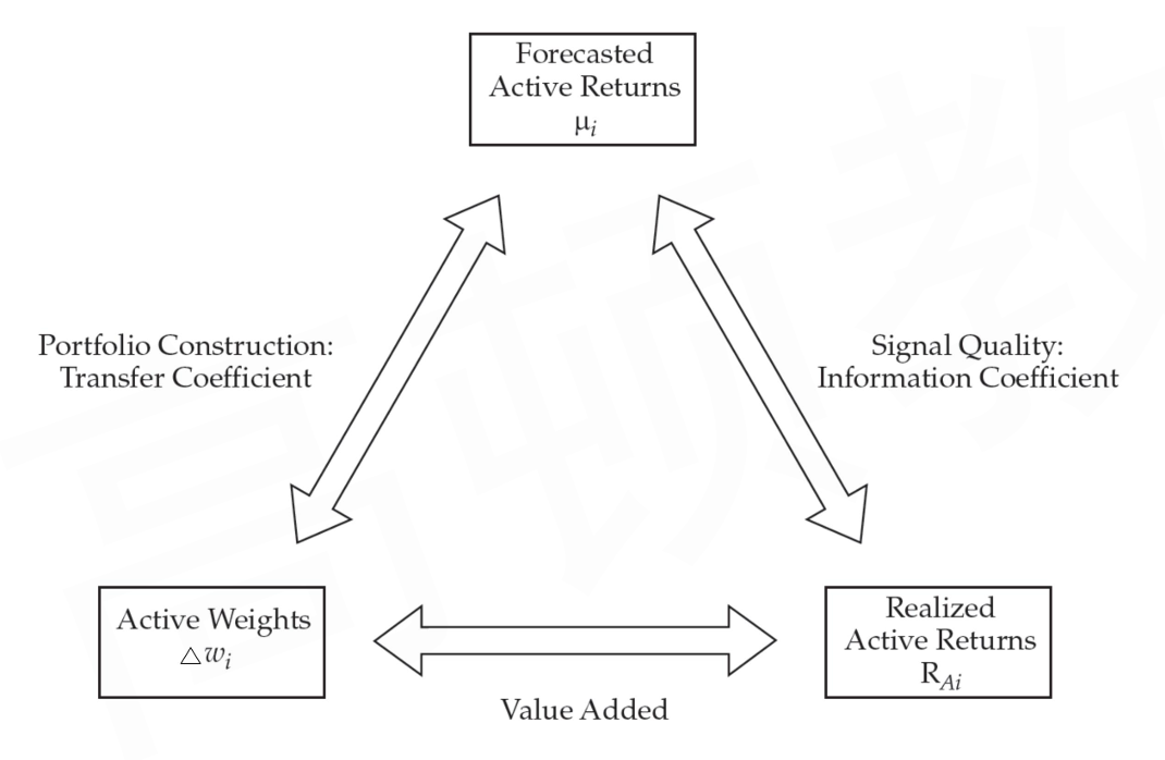
The Correlation Triangle
Information Coefficient
Signal quality is measured by the correlation between the forecasted active returns (\mu_i) at the top of the triangle and the realized active returns (R_{A,i}) at the right corner, commonly called the information coefficient(IC)
IC is a risk-weighted correlation between the active returns and the realized active returns
IC=\rho\left(\frac{R_{A,i}}{\sigma_i},\frac{\mu_i}{\sigma_i}\right)
Ex-ante IC usually be positive
Ex-post IC may be positive or negative
Transfer Coefficient
The correlation between any set of active weights (\Delta w_i) in the left corner, and forecasted active returns (\mu_i) at the top of the triangle,measures the degree to which the investor's forecasts are translated into active weights, called the transfer coefficient (TC)
TC is a correlation between the forecasted active security returns and actual active weights
TC=\rho\left(\frac{\mu_i}{\sigma_i},\Delta w_i\sigma_i\right)
The degree to which the investor's forecasts are translated into active weights
The extent to which constraints reduce the expected value added of the investor's forecasting ability
For portfolios without any constraints → TC = 1
For portfolios with constraints → TC < 1
Basic and Full Fundamental Law
Breadth
Breadth(BR) measures the number of independent active decisions make per year by the manager in constructing the portfolio, which is an indicator of how much efforts the manager has put into
"Independent" means that the active decisions should not be based on highly correlated (or identical) information sets
A practical measure of breadth: BR=\frac{N}{1+(N-1)\rho}
when using derivatives or other forms of hedging strategies (\rho\lt 0),BR may be larger than N
The Fundamental Law
The basic fundamental law IR=IC\times\sqrt{BR} E(R_A)=IR\times\sigma_A=IC\times\sqrt{BR}\times\sigma_A
The full fundamental law IR=TC\times IC\times\sqrt{BR} E(R_A)=IR\times\sigma_A=Tc\times IC\times\sqrt{BR}\times\sigma_A
When take"TC" into consideration: \sigma_A^\ast=\sigma_{(R_P-R_B)}^\ast=\frac{TC\times IR}{SR_B}\times\sigma_{R_B} SR_P^2=SR_B^2+(TC\times IR)^2
Application of the Fundamental Law
Market Timing
Market timing simply bets on the market direction
Information coefficient can be used for inferring market timing
IC = 2 × (% correct)-1
If the manager is correct 50% of the time, then IC = O
This formula is also applicable to evaluate IC of active sector rotation strategies
Most of the fundamental law perspectives discussed up to this point relate to the expected value added through active portfolio management
Expected value added conditional on the realized information coefficient:
Actual performance in any given period will vary from its expected value E(R_A)=TC\times IC\times\sqrt{BR}\times\sigma_A E(R_A\mid IC_{\text{realized}})=TC\times IC_{\text{realized}}\times\sqrt{BR}\times\sigma_A R_A=E(R_A\mid IC_{\text{realized}})+\text{Noise}
An ex-post (i.e. realized) decomposition of the portfolios active return variance into two parts
Variation due to the realized information coefficient (TC^2)
Variation due to constraint-induced noise(1-TC^2)
Limitations of the Fundamental Law
Poor input estimates lead to incorrect evaluation
Uncertainty in ex-ante measurement of skill
IC is difficult to justify due to existence of the bias, various asset segments, or different time periods
Assumption of independence of active decisions
The number of individual assets is not an adequate measure of strategy breadth (BR) when the active returns between individual assets are correlated