Forward Commitments
Forwards Contracts
General Formula
- No-Arbitrage Principle
- The no-arbitrage principle: determine the price of a derivative by assuming that there are no arbitrage opportunities
The portfolio should yield the risk-free rate of return if it generates certain payoffs
The investor can be assumed to be risk neutral, because the investor's risk aversion is not a factor in determining the derivative price - Virtually all derivative pricing models ultimate take this form:
Discounting the expected payoff of the derivative at the risk-free rate
- The no-arbitrage principle: determine the price of a derivative by assuming that there are no arbitrage opportunities
- Pricing of Forwards Contracts
- If the underlying asset generates no periodic cash flows, the forwards' price can be calculated as follows:
F_0(T)=S_0\times\left(1+r_f\right)^{T}
S_0 is spot price of the underlying asset
r_f is risk-free rate
T is the time span from now to expiration
- If the underlying asset generates no periodic cash flows, the forwards' price can be calculated as follows:
- Valuation of Forwards Contracts
- At initiation
V_{L,0}=V_{S,0}=0 - At expiration
V_{L, T}=S_T-F_0(T)
V_{S, T}=F_0(T)-S_T - During its life (t < T)
V_{L, t}=S_t-\frac{F_0(T)}{\left(1+r_f\right)^{T-t}}=\frac{F_t(T)-F_0(T)}{\left(1+r_f\right)^{T-t}}
V_{S, t}=\frac{F_0(T)}{\left(1+r_f\right)^{T-t}}-S_t=\frac{F_0(T)-F_t(T)}{\left(1+r_f\right)^{T-t}}
- At initiation
- With Benefits and Costs
- Benefits will decrease forwards' price at initiation
Dividend
Coupon
Rents revenue
Convenience yield: nonmonetary advantage of holding the asset - Costs will increase forwards' price at initiation
Storage cost
Maintenance cost - Pricing
F_0(T)=\left(S_0-P V B+P V C\right) \times\left(1+r_f\right)^{T}=S_0\times\left(1+r_f\right)^{T}-FVB+FVC - Valuation
V_{L, T}=S_T-F_0(T)
V_{S, T}=F_0(T)-S_T
V_{L, t}=\left(S_t-P V B_t+P V C_t\right)-\frac{F_0(T)}{\left(1+r_f\right)^{T-t}}
V_{S, t}=\frac{F_0(T)}{\left(1+r_f\right)^{T-t}}-\left(S_t-P V B_t+P V C_t\right)
- Benefits will decrease forwards' price at initiation
Fixed-Income Forwards and Equity Forwards
- Pricing and Valuation of Fixed-Income Forwards
- The price of fixed-income forwards
F_0(T)=\left(S_0-\text { PVCoupon }\right) \times\left(1+r_f\right)^{T}
F_0(T)=S_0\times\left(1+r_f\right)^{T}-\text { FVCoupon } - The value of fixed-income forwards
V_{L, t}=\left(S_t-\text { PVCoupon }_t\right)-\frac{F_0(T) }{\left(1+r_f\right)^{T-t}}=\frac{F_t(T)-F_0(T)}{\left(1+r_f\right)^{T-t}}
V_{S, t}=\frac{F_0(T) }{\left(1+r_f\right)^{T-t}}-\left(S_t-\text{ PVCoupon }_t\right)=\frac{F_0(T)-F_t(T)}{\left(1+r_f\right)^{T-t}}
- The price of fixed-income forwards
- Pricing and Valuation of Stock Forwards
- The price of stock forwards
F_0(T)=\left(S_0-\text { PVDivdend }\right) \times\left(1+r_f\right)^{T}
F_0(T)=S_0\times\left(1+r_f\right)^{T}-\text { FVDivdend } - The value of fixed-income forwards
V_{L, t}=\left(S_t-\text { PVDivdend }_t\right)-\frac{F_0(T) }{\left(1+r_f\right)^{T-t}}=\frac{F_t(T)-F_0(T)}{\left(1+r_f\right)^{T-t}}
V_{S, t}=\frac{F_0(T) }{\left(1+r_f\right)^{T-t}}-\left(S_t-\text{ PVDivdend }_t\right)=\frac{F_0(T)-F_t(T)}{\left(1+r_f\right)^{T-t}}
- The price of stock forwards
- Pricing and Valuation of Equity Index Futures
- The price of equity index futures
F_0(T)=S_0\times e^{(r_f^c-\delta^c)\times T}
r_f^c is continuously compounded risk-free rate
\delta^c is continuously compounded dividend yield - The value of equity index futures
V_{L, t}=S_t \times e^{-\delta^c \times(T-t)}-F_0(T) \times e^{-r_f^c \times(T-t)}
V_{S, t}=F_0(T) \times e^{-r_f^c \times(T-t)}-S_t \times e^{-\delta^c \times(T-t)}
- The price of equity index futures
Forward Rate Agreement
- Pricing of FRA
- Forward rate models show how forward rates can be extrapolated from spot rates
1+\mathrm{S}_{\mathrm{b}} \times \frac{30\times \mathrm{b}}{360}=\left(1+\mathrm{S}_{\mathrm{a}} \times \frac{30\times \mathrm{a}}{360}\right) \times\left(1+\mathrm{FR} \times \frac{30\times(\mathrm{b}-\mathrm{a})}{360}\right)
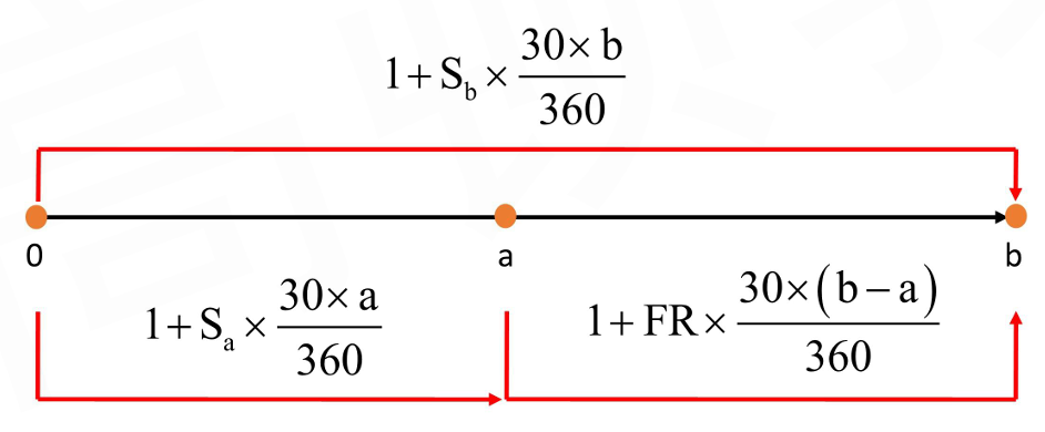
- Forward rate models show how forward rates can be extrapolated from spot rates
- Valuation of FRA at Expiration
{V}_{{L}, {T}}=\frac{A \times(S_{b-a}- {FR }) \times\frac{ { b-a }}{360}}{1+S_{b-a} \times\frac{ { b-a }}{360}}- For "axb FRA", the "interest saving" due to the FRA position comes at "Time b", but is settled at "Time a"
- So the "interest saving" need to be discounted to "Time a" to calculate the value of FRA
- Valuation of FRA Prior to Expiration
- calculate the new FRA rate
1+S_{b-t}\times\frac{b-t}{360}=\left(1+S_{a-t}\times\frac{a-t}{360}\right)\times\left(1+FR_t\times\frac{b-a}{360}\right) - calculate the value of FRA for the long position
{V}_{{L}, {T}}=\frac{A \times(FR_t- FR_0 ) \times\frac{ { b-a }}{360}}{1+S_{b-t} \times\frac{ { b-t }}{360}}
- calculate the new FRA rate
Fixed Income Futures
- A fixed-income futures contract has more than one bond that can be delivered by the short (delivery option)
- A basket of deliverable bonds: $100,O0O par value T-bonds with any coupon but with a maturity of at least 15 years
The quotes for T-bonds are in points and 32nds: A price quote of 95-18 is equal to 95.5625 and a dollar quote of $95,562.50 - The underlying asset is a hypothetical 30 year treasury bond with 6% coupon rate
- A basket of deliverable bonds: $100,O0O par value T-bonds with any coupon but with a maturity of at least 15 years
- Conversion factor (CF) is used in an effort to make all deliverable bonds roughly equal in price
- Principal invoice amount = Quoted futures price x CF
- The futures contract seller will receive the following at delivery
- Total invoice amount = principal invoice amount + accrued interest
- When multiple bonds can be delivered for a futures contract with particular maturity, a cheapest-to-deliver(CTD) bond typically emerges after adjusting for the conversion factor
- Quoted futures price
\text{Quoted futures price}=\frac{\left(S_0-P V C\right) \times\left(1+r_f\right)^{T}-A I_T}{CF}=\frac{S_0 \times\left(1+r_f\right)^{T}-A I_T-FVC}{CF}- S_0: T-bond''s spot full price
S_0=\text{quoted price(T-bond's clean price)}+AI_0 - AI_T: the accrued interest at maturity of the futures contract
- CF: the conversion factor
- S_0: T-bond''s spot full price
Swaps Contracts
Interest Rate Swaps
- Pricing of Interest Rate Swap
- The fixed rate in a plain vanilla swaps contract (swap rate) should makes the contract value zero at initiation
- A plain vanilla swaps contract can be viewed as the combination of two bonds (long + short)
- \text{Fix Rate}=\frac{1-DF_n}{DF_1+DF_2+\cdots+DF_n}
- Valuation of Interest Rate Swaps
- The value of a swap is the difference of value between the floating-rate bond and the fixed-rate bond at any time during the life of the swap
- At each settlement date, the coupon rate of a floating rate will be reset to the market rate, so the value of a floating rate bond will be equal to the par value
Currency Swaps
- Pricing of Currency Swaps
- The fixed rate in a currency swap is simply the swap rate calculated from the spot rates of the corresponding currency
- \text{Fix Rate}=\frac{1-DF_n}{DF_1+DF_2+\cdots+DF_n}
- Valuation of Currency Swaps
- Calculate the fixed and/or floating rate bond prices in both currencies
- Adjust currency to the same one
- The value of a swaps contract is the difference of value (in same currency) between the two equivalent bonds
Equity Swaps
- An equity swap contract is a derivative contract in which two parties agree to exchange a series of cash flows whereby 铁幕 is exchanged with fixed rate/floating rate/another equity return
- The equity return could be from an equity index, a single stock, or a basket of stocks
- Notional amount is not exchanged at the beginning or the end of the swap
- On settlement dates, payments are netted
- The pricing issue is only for "equity return vs. fixed rate"
- A total return swaps contract is a slightly modified equity swap
- It includes in the performance any dividends paid by the underlying stocks or index during the period until the swap maturity
- Pricing of Equity SwapS
- The pricing of equity swap is similar to that of interest rate swaps,we can use the same formula to calculate the fixed rate
- \text{Fix Rate}=\frac{1-DF_n}{DF_1+DF_2+\cdots+DF_n}
- Valuation of Equity Swaps
- For receive fixed rate, pay equity return swaps
V_t=P V_{\text {Fixed-rate bond }}-\left(S_t / S_{t-}\right) \times N P - For receive floating rate, pay equity return swaps
V_t=\left(S_t / S_{t-}\right) \times N P-P V_{\text {Fixed-rate bond }} - For receive equity(1) return, pay another equity(2) return swaps
V_t=\left(S_{1, t} / S_{1, t-}\right) \times N P-\left(S_{2, t} / S_{2, t-}\right) \times N P=\left(R_1-R_2\right) \times N P
- For receive fixed rate, pay equity return swaps
Contingent Claims
Binomial Model
Components of Binomial Option Valuation Model
- Components of Binomial Option Valuation Model
- The beginning asset value (S_0)
- The size of the two possible changes (U, D)
- The probabilities of each of these changes occurring (\pi_U,\pi_D)
- Risk-Neutral Probability
- In a risk-neutral world, investors require no compensation for risk,and the expected return on all securities is the risk free rate
- Risk-neutral probability of up-move
\pi_{\mathrm{u}}=\frac{\left(1+\mathrm{r}_{\mathrm{f}}\right)^{\mathrm{T}}-\mathrm{D}}{\mathrm{U}-\mathrm{D}} - Risk-neutral probability of down-move
\pi_{\mathrm{d}}=1-\pi_{\mathrm{u}}=\frac{\mathrm{U}-\left(1+\mathrm{r}_{\mathrm{f}}\right)^{\mathrm{T}}}{\mathrm{U}-\mathrm{D}}
One-Period Binomial Model
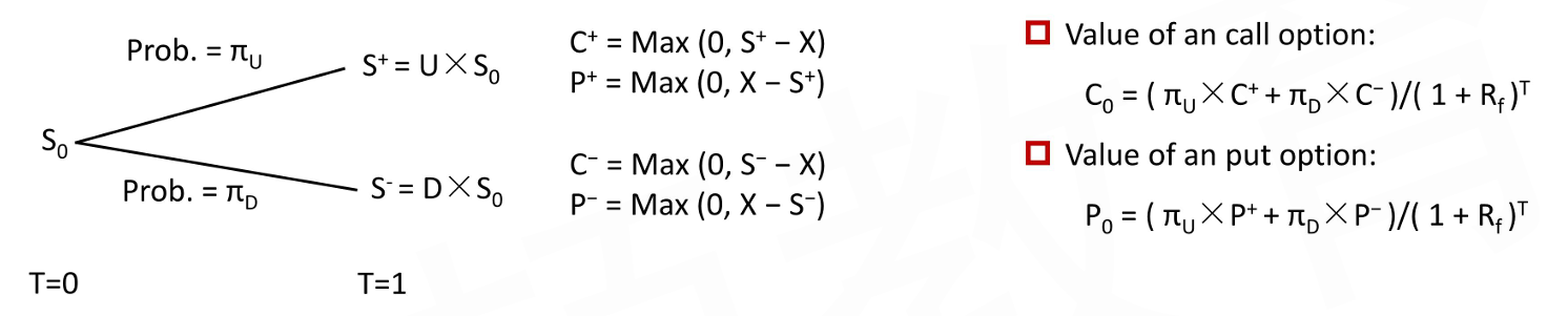
- Calculate the payoff of the option at maturity in both the up-move and down-move states
- Calculate the expected value of the option in one period as the probability-weighted average of the payoffs in each state
- Discount this expected value back to today at the risk-free rate
More Understanding of Risk-Neutral Probability
- The Risk-Neutral Valuation
- Construct an arbitrage-free portfolio consisting of H shares of stocks and one short call
he current value of the portfolio is: V=H \times S-C - One period later (assume one year here), the value will go to either {V}^{+} or {V}^{-}
\mathrm{V}^{+}={H} \times {S}^{+}-{C}^{+}\quad {V}^{-}={H} \times {S}^{-}-{C}^{-} - Choose the value of H to make the portfolio be a hedged portfolio
\mathrm{V}^{+}={V}^{-} \rightarrow {H} \times {S}^{+}-{C}^{+}={H} \times {S}^{-}-{C}^{-} - We then solve for H to obtain:
Hedge ratio H=\frac{{C}^{+}-{C}^{-}}{{S}^{+}-{S}^{-}}=\frac{{C}^{+}-{C}^{-}}{{S} \times {U}-{S} \times {D}} - The portfolio then becomes a risk-free portfolio and should generate the risk-free rate:
V^{+}=V^{-}=V \times\left(1+R_f\right) - We then solve for C to obtain
C=\frac{\pi \times C^{+}+(1-\pi) \times C^{-}}{1+R_f}
- Construct an arbitrage-free portfolio consisting of H shares of stocks and one short call
- The price of call option today is a weighted average of two call prices next period discounted at the risk-free rate
- The weights are \pi and 1-\pi, which are known as risk-neutral probabilities
Arbitrage Opportunity Involving Options
- If the option market price is different from the calculated price from the binomial valuation model, an arbitrage opportunity exist
- If market price > calculated price, sell the call option and buy H shares of the stock for each option we sold
- If market price < calculated price, buy the call option and sell H shares of the stock for each option we bought
Interest Rate Option
- Binomial Interest Rate Tree
- A binomial interest rate tree model that assumes interest rates at any point of time (node) have an equal probability of taking one of two possible values in the next period, an upper path (U) and a lower path (L)
- Interest rates are different in different periods of time
- Binomial Valuation Model for Interest Rate Option
- Call payoff = Max(0, underlying rate - exercise rate ) × NP
- Put payoff = Max(0, exercise rate - underlying rate ) × NP
BSM Model
Initial Model
- Continuous-Time Option Pricing Model
- As the period covered by a binominal model is divided into arbitrarily small discrete time periods, the model results converge to those of continuous-time model
- The famous Black-Scholes-Merton model (BSM model) values options in continuous-time and is derived from the same no-arbitrage assumption used to value the binominal model
- Assumptions of BSM Model
- The options are European-style
- The underlying asset price follows a geometric Brownian motion, and moves smoothly from value to value
- The continuously compounded risk-free interest rate is known and constant
Borrowing and lending at the risk-free rate is allowed - The volatility of the underlying asset return is constant and known
- The market is frictionless
No transaction costs, no taxes, no regulatory constraints
No-arbitrage opportunities in the market
The underlying asset is highly liquid, and continuous trading is available
Short selling of the underlying asset is permitted
- More Interpretations
- Call option can be regarded as leveraged stock investment
Borrow money to invest in the stock - Put option can be regarded as combination of long bond and short stock
Buy the bond (lend money) with the proceeds from short selling stock
- Call option can be regarded as leveraged stock investment
- Carrying Benefits or CostS
- Carry benefits include
Dividends for stock
Foreign interest rates for currency - Carry costs include
Storage cost
Insurance costs - Carry costs can be treated as negative carry benefits
- Carry benefits include
Black Model
- Option on Futures
- lgnore margin requirements and marking to market for futures
- The option on futures expires on the delivery date of the underlying futures contract
\begin{align} &c_0=e^{-r_fT}\left[FN(d_1)-XN(d_2)\right] \\ &p_0=e^{-r_fT}\left[XN(-d_2)-FN(-d_1)\right] \\ &d_{1,2}=\frac{\ln\left({F/X}\right)}{\sigma\sqrt T}\pm \frac{\sigma\sqrt T}{2} \end{align}
F_0(T) is the futures price at Time 0 that expires at Time T
\sigma denotes the volatility related to the futures price
- Interest Rate Option
- Assume a "m × n" structure, and the formula for options are as follows
\begin{align} &c_0=Ae^{-\frac{nr_f}{360}}\left[f_{m,n}N(d_1)-XN(d_2)\right]\times\frac{n-m}{360} \\ &p_0=Ae^{-\frac{nr_f}{360}}\left[XN(-d_2)-f_{m,n}N(-d_1)\right]\times\frac{n-m}{360} \end{align}
- Assume a "m × n" structure, and the formula for options are as follows
- Swaption
- A swaption is an option to enter into a swap
- A payer swaption is an option to enter into a swap as the fixed-rate payer
If interest rate increases, the payer swaption value will go up
A payer swaption is equivalent to a call option on floating rate - A receiver swaption is an option to enter into a swap as the fixed-rate receiver (the floating-rate payer)
If interest rate increases, the receiver swaption value will go down
A receiver swaption is equivalent to a put option on floating rate - Black Model for Swaption
\begin{align} &V_{payer}=A\times\text{Accrual Period}\times\text{PVA}\times\left[r_{fix}N(d_1)-r_{X}N(d_2)\right] \\ &V_{receiver}=A\times\text{Accrual Period}\times\text{PVA}\times\left[r_{X}N(-d_2)-r_{fix}N(-d_1)\right] \end{align}
r_{fix} is the forward swap rate
r_X the exercise swap rate
PVA is present value of an annuity matching the forward swap payment
Option Greeks
- The relationship between each input and the European option price is captured by a sensitivity factor called the option Greeks
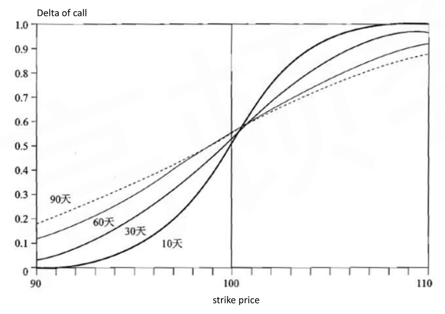
- Delta(\Delta): option price vs. underlying price (S)
- Gamma(\Gamma): delta vs. underlying price(S)
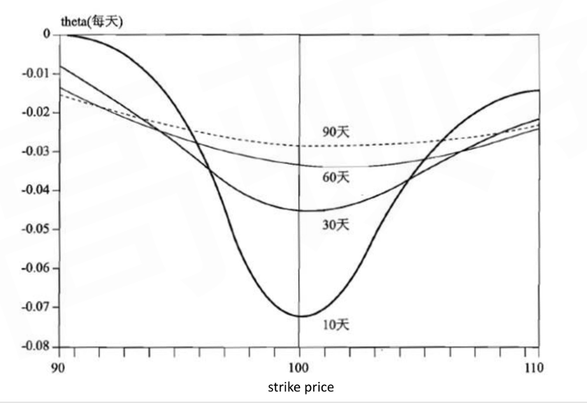
- Theta(\theta): option price vs. time passage (t)
- Vega(\Lambda): option price vs. underlying price volatility(\sigma)
- Rho(\rho): option price vs. risk free rate (r_f)
- Delta
- For non-dividend-paying stock
\Delta_{call}=N(d_1),\Delta_{put}=-N(-d_1) - For dividend-paying stock
\Delta_{call}=e^{-\delta T}N(d_1),\Delta_{put}=-e^{-\delta T}N(-d_1) - \Delta_{call} increases from 0 to 1 as stock price increases
\Delta_{put} increases from -1 to 0 as stock price increases
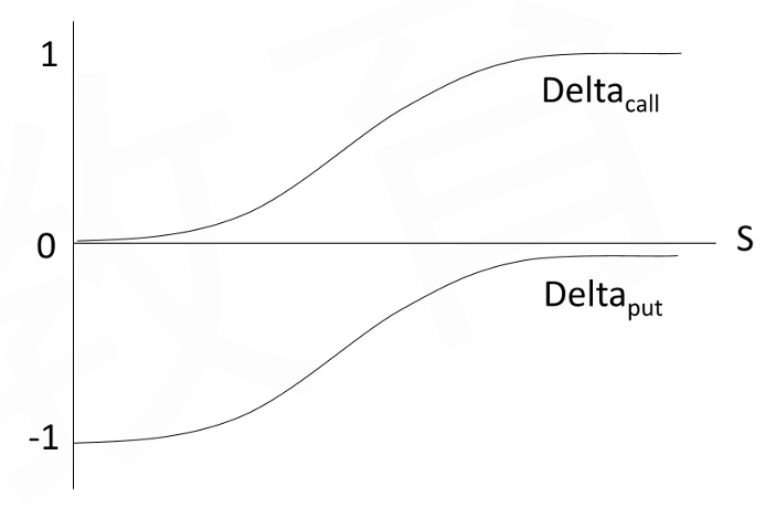
- When the call (put) option gets closer to maturity, the delta will drift either toward O if it is out-of-the-money or drift toward 1(-1) if it is in-the-money
- Delta-neutral portfolio by delta-hedging means combining the option position with a position in the underlying asset to form a portfolio, whose value does not change in reaction to changes in the price of the underlying over a short period of time
The delta-neutral hedging is a dynamic process, since the delta is constantly changing
- For non-dividend-paying stock
- Gamma
- Gamma is the sensitivity of the option's delta against the underlying asset price
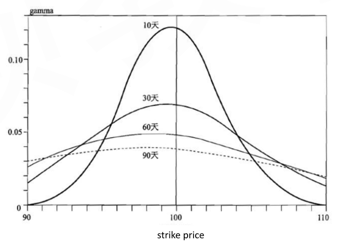
Gamma is largest when the option is at-the-money, and approaches zero if the option is deep in- or out-of-the-money
Gamma increases as expiration approaches - Gamma for a call and put option with identical features are the same
Long call (put) will have a positive gamma
Short call (put) will have a negative gamma - Delta-neutral positions can hedge the portfolio against small changes in stock price, while gamma can help hedge against relatively large changes in stock price
In some cases, adding other options to current positions would make the gammas offset (gamma hedge) - Gamma risk: stock prices often jump rather than move continuously and smoothly in reality, holding a delta-neutral portfolio will have risk against stock price too
- Gamma is the sensitivity of the option's delta against the underlying asset price
- Theta
- Theta is the sensitivity of the option price against time passage
- Theta affects the value of put and call options in a similar way
- As time passes, most call and put options decrease in value, so theta is usually negative for both call and put option
With exception to deep in-the-money put option - Theta varies with changes in stock prices and as time passes
Theta is most pronounced when the option is at-the-money
Theta usually increases in absolute value as expiration approaches
- Vega
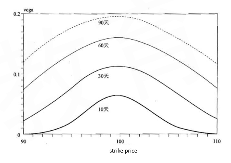
- Vega is the sensitivity of option price against the volatility of the underlying asset price
- Vegas are the same for call and put option with identical features
- Vega is always positive
- Vega is high when options are at or near the money
- Historical volatility is using historical data to calculate the variance and standard deviation of the continuously compounded returns
- We can set the BSM price equal to the market price and then work backwards to get the volatility, this volatility is called the implied volatility
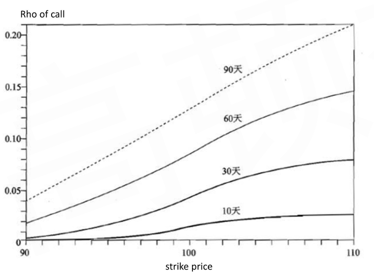
- Rho
- Rho is the sensitivity of option price against the risk-free rate
- Rho is positive for call option
- Rho is negative for put option