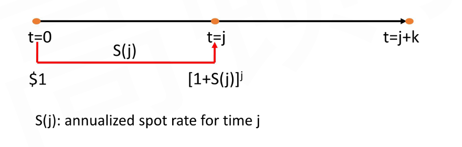
Spot rate is the rate of interest on a security that makes a single payment at a future point in time
The annualized return (also can be interpreted as the yield to maturity) on an option-free and default-risk-free zero-coupon bond
Also known as zero-coupon rate or zero rate
Spot Curve
Spot curve: the term structure of spot rates, the graph of the spot rate versus maturity
The shape and level of the spot yield curve are dynamic
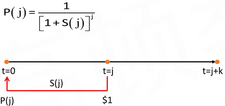
Discount Factor
It is the price of a risk-free single-unit payment at time j
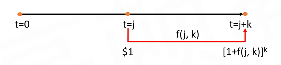
Forward Rate
Forward rate is the rate of interest set today for a single-payment security to be issued at a future date
f(j, k): annualized k-year forward rate starting at time j
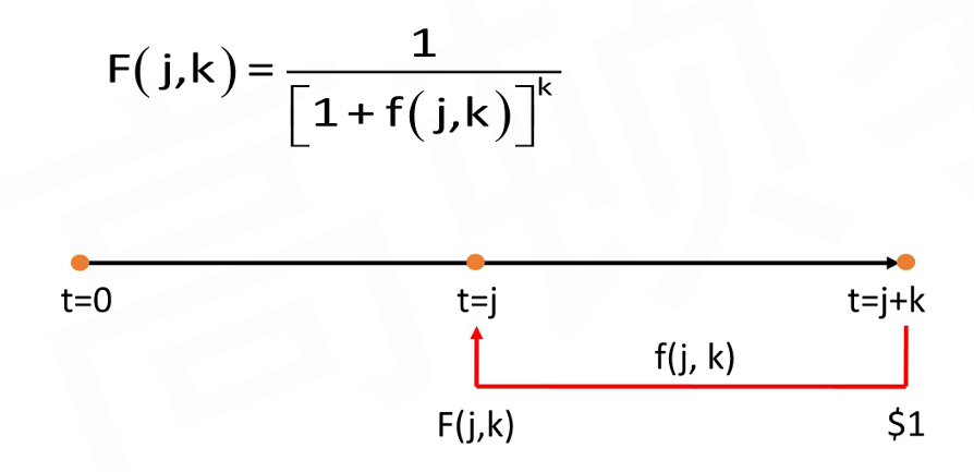
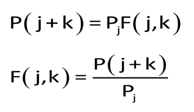
Discount Factor
The price at time j years from today for a zero-coupon bond with maturity (j+k) years and unit principal
Forward Rate Curve
The term structure of forward rates, the graph of the forward rate versus maturity
It represents the term structure of forward rates for a loan made on a specific initiation date
Forward Rate Models
Forward rate models show how forward rates can be extrapolated from spot rates
Forward Pricing Model
The forward pricing model describes the valuation of forward contracts
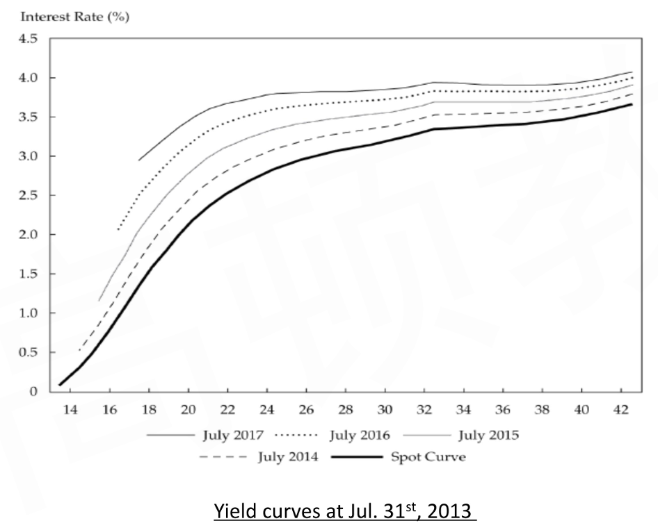
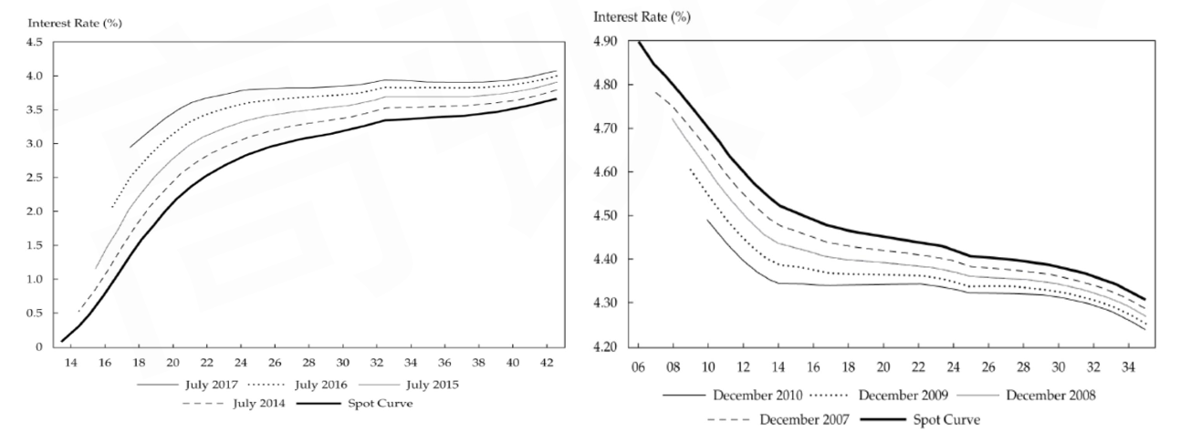
Spot Curve vs. Forward Curve
If the spot curve is upward sloping, forward curves lie above the spot curve
The later the initiation date, the higher the forward curve
If the spot curve is downward sloping, forward curves lie below the spot curve
The later the initiation date, the lower the forward curves
Yield Curve Shapes
In developed markets, yield curves are most commonly upward sloping with diminishing marginal increases in yield for identical changes in maturity
An inverted yield curve is uncommon and such term structure may reflect a market expectation of declining future inflation rates
A flat yield curve typically occurs briefly in the transition from an upward-sloping to a downward-sloping yield curve, or vice versa.
A humped驼峰 yield curve, which is relatively rare, occurs when intermediate-term interest rates are higher than short- and long-term rates
Par Rate
Par Rate and Par Curve
Par rate is the coupon rate for bond that would result in bond price equals to its par value
Par curve represents the yields to maturity/coupon rate/par rate on coupon-paying government bonds, priced at par, over a range of maturities
Recently issued("on the run") bonds are typically used to create the par curve because new issues are typically priced at or close to par
Bootstrapping
Spot rates may be obtained from the par curve by bootstrapping
YTM
YTM is the internal rate of return of on the cash flow, it reflects the implied single market discount rate
For coupon bonds, if the spot curve is not flat, the YTM will not be the same as the spot rate
YTM is the same as the spot rate for zero-coupon bonds
YTM is some weighted average of spot rates
Expected Return vs. Realized Return
Expected return is the ex-ante return that a bondholder expects to earn
The YTM is the expected return and will be realized only if all the three critical assumptions for YTM are met
Realized return is the actual return on the bond during the time an investor holds the bond
It is based on actual reinvestment rates and the yield curve at the end of the holding period
The YTM can provide a poor estimate of expected return if:
interest rates are volatile
the yield curve is steeply sloped, either upward or downward
there is significant risk of default
the bond has one or more embedded options (e.g., put, call, or conversion)
Implicit in the determination of the yield to maturity as a potentially realistic estimate of expected return is a flat yield curve
Swap Rate
Swap rate is the interest rate for the fixed-rate leg of an interest rate swap
Determining swap rate
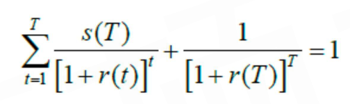
The right side is the value of the floating leg, which is 1 at origination
The swap rate is determined by equating the value of the fixed leg, on the left-hand side to the value of the floating rate
Swap Curve
The yield curve of swap rates is called the swap rate curve (swap curve)
Because it is based on so-called par swaps, the swap curve is a type of par curve
Swap Curves vs Government Spot Curves
The swap market has more maturities
Many countries do not have a liquid government bond market with maturities longer than one year
The swap market is a highly liquid market
Unlike bonds, a swap does not have multiple borrowers or lenders, only counterparties who exchange cash flows
Swaps provide one of the most efficient ways to hedge interest rate risk
Swap rates reflect the credit risk of commercial banks rather than governments
Swap market is unregulated (not controlled by governments),so swap rates are more comparable across different countries
Spread
Swap Spread
Swap spread is the amount by which the swap rate exceeds the rate of the "on-the-run" government security with the same maturity
Swap spread = swap rate - government security rate
Swap spread shows the Treasury rate can differ from the swap rate for the same term
Unlike the cash flows from US Treasury bonds, the cash flows from swaps are subject to much higher default risk
Market liquidity for any specific maturity may differ: some parts of the term structure of interest rates may be more actively treaded with swaps than with Treasury bonds
I- Spread
I-spreads are the bond rates net of the swap rates of the same maturities
I-spread = bond rate - swap rate
I-spread reflects compensation for credit and liquidity risks
TED Spread
The TED spread is calculated as the difference between Libor and the yield on a T-bill of matching maturity
TED = LIBOR - T-bill rate
TED spread is an indicator of perceived credit risk in the general economy
TED spread can also be thought of as a measure of counterparty risk
TED spread more accurately reflects risk in the banking system
An increase in the TED spread is a sign that lenders believe the risk of default on interbank loans is increasing
Libor-OIS Spread
Libor-OIS spread is the difference between Libor and the overnight indexed swap(OIS) rate
OIS is an interest rate swap in which the periodic floating rate is equal to the geometric average of an overnight index rate over every day of the payment period
The Libor-OlS spread is considered an indicator of the risk and liquidity of money market securities
Z-Spread
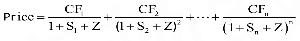
Z-spread is the constant spread that would need to be added to the implied spot curve so that the discounted cash flows of a bond are equal to its current market price
Implied assumption: the yield curve makes a parallel shift
Under the assumption of zero interest rate volatility, it is not appropriate for bonds with embedded options
Term Structure Theories
Pure Expectation Theory/Unbiased Expectation Theory
Pure expectation theory suggests that the forward rate is an unbiased predictor of the future spot rate
If yield curve is upward sloping, short-term rates are expected to rise
If yield curve is downward sloping, short-term rates are expected to fall
If yield curve is flat, short-term rates are expected to remain constant
Its interpretation is that bonds of any maturity are perfect substitutes for one another
The predictions of the unbiased expectations theory are consistent with the assumption of risk neutrality
This assumption is a significant shortcoming because investors are risk averse
Local Expectation Theory
Local expectation theory assumes risk-neutrality only in the short term while incorporate uncertainty in the long term
Under this theory, the expected return for every bond over short time periods is the same
But it is often observed that short-holding-period returns on long-dated bonds do exceed those on short-dated bonds
The need for liquidity and the ability to hedge risk essentially ensure that the demand for short-term securities will exceed that for long-term securities
Liquidity Preference Theory
Liquidity preference theory asserts that liquidity premiums exist to compensate investors for the added interest rate risk they face when lending long term Forward rate = expected from spot rates + liquidity premium
Liquidity premium increase with maturity
Segmented Markets Theory
Under segmented markets theory, each maturity sector can be thought of as a segmented market in which yield is determined by supply of and demand for loan, and independent from the yields in other maturity segments
Consistent with a world where there are asset-liability management constraints
Yields are not a reflection of expected spot rates or liquidity premiums
Preferred Habitat Theory
Preferred habitat theory contends that if the premium is large enough, investor will deviate from their preferred maturities or habitats
Premium is not directly related to maturity
Based on the realistic notion that investors will accept additional risk in return for additional expected returns
Yield Curve Factor Models
Yield Curve Movement
The yield curve movements can be decomposed into
parallel movement (\Delta X_L)
steepness movement (\Delta X_S)
curvature movements (\Delta X_C)
Parallel shift(level) → effective duration
Changes in Level rates 77%
Non-parallel shift → key rate duration
Steepness: Slope changes 17%
Curvature: Curvature changes 3%
Yield Curve Risk
Yield curve risk (Shaping risk) is the risk to portfolio value arising from unanticipated changes in the yield curve
Effective duration: measures the sensitivity of a bond's price to a small parallel shift in a benchmark yield curve Address risk associated with parallel yield curve changes
key rate duration: measures a bond's sensitivity to a small change in a benchmark yield curve at a specific maturity segment Allows identification and management of "shaping risk"
Decompose the Risk
The proportional change in portfolio value resulted from yield curve movement can be modeled as:
\frac{\Delta P}{P} \approx-D_L \Delta X_L-D_S \Delta X_S-D_C \Delta X_C
D_L, D_S, and D_C as the sensitivities of portfolio value to small changes in the level, steepness, and curvature, respectively
Key Rate Duration
Key rate duration measures the bond price sensitivity to a small change in a benchmark yield curve at a specific maturity segment
Effective duration is an adequate measure of bond price risk only for small paralleled shifts in the yield curve
For the portfolio that is composed by zero-coupon bonds:
A representation of the yield volatility of a zero-coupon bond for every maturity of security
The volatility term structure typically shows that short-term rates are more volatile than long-term rates Short-term volatility is most strongly linked to uncertainty regarding monetary policy Long-term volatility is most strongly linked to uncertainty regarding the real economy and inflation
On the basis of the typical assumption of a lognormal model, the uncertainty of an interest rate is measured by the annualized standard deviation of the proportional change in a bond yield over a specified time interval
Active Bond Portfolio Management
Strategy of Forward Contract
Forward contract's price is settled today
Forward contract's value remains unchanged as long as future spot rates evolve as predicted by today's forward rate
A change in the forward contract's value reflects a deviation of the future spot rates from that predicted by today's forward rate
An active portfolio manager may outperform the overall market if the manager can predict how future spot rates will differ from the current implied forward rates
If a trader expects that the future spot rate will be lower than what is predicted by the prevailing forward rate
The forward contract value is expected to increase
The trader would long the forward contract
If a trader expects the future spot rate to be higher than what is predicted by the existing forward rate
The forward contract value is expected to decrease
The trader would short the forward contract
Riding the Yield Curve
When a yield curve is upward sloping and the trader believes that the yield curve will not change its level and shape, then buying bonds with a maturity longer than the investment horizon would provide a total return greater than the return on a maturity-matching strategy
When the yield curve slopes upward, as a bond approaches maturity or "rolls down the yield curve", it is valued at successively lower yields and higher prices
Macroeconomic Variables
Bond Risk Premium
Interest rate dynamics are influenced by key economic variables and market events
The bond risk premium (a.k.a. term (or duration) premium) refers to the expected excess return of a default-free long-term bond less that of an equivalent short-term bond or the one-period risk-free rate
Unlike ex post observed historical returns, the bond risk premium is a forward-looking expectation and must be estimated
Macroeconomic Factors Influence
Several macroeconomic factors influence bond pricing and required returns
Research shows that inflation explains about two-thirds of long-term bond yield variation,with the remaining third roughly equally attributable to economic growth and factors including monetary policy
Monetary policy explains nearly two-thirds of short-and intermediate-term yield variation, and the remaining third is largely attributable to inflation
Monetary policy
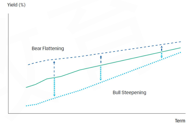
During economic expansions, monetary authorities raise benchmark rates to help control inflation, and this action is often consistent with bearish flattening,or short-term bond yields rising more than long-term bond yields, resulting in a flatter yield curve
During economic recessions or anticipated recessions,the monetary authority cuts benchmark rates to help stimulate economic activity, and the lowering of interest rates is associated with bullish steepening, in which short-term rates fall by more than long-term yields, resulting in a steeper term structure
Fiscal policy
Fiscal supply-side effects affect bond prices and yields by increasing(decreasing) yields when budget deficits rise(fall)
Longer government debt maturity structures predict greater excess bond returns
This is effectively a segmented market factor, wherein the greater supply of bonds of long-term maturity increases the yield in that market segment
Investor Demand
Domestic investor demand is a key driver of bond prices
Greater domestic investor demand increases prices and reduces the bond risk premium
Non-domestic investor demand influences government bond prices and may result either from holding reserves or from actions associated with currency exchange rate management
Non-domestic flows significantly influence bond prices because inflows (outflows) bid up (down) bond prices, lowering (raising) the bond risk premium
Investor Strategies
During highly uncertain market periods, investors flock to government bonds in what is termed a flight to quality
A flight to quality is often associated with bullish flattening, in which the yield curve flattens as long-term rates fall by more than short-term rates
An investor may seek to capitalize on an expected bullish flattening of the yield curve by shifting from a bullet to a barbell position
Investors expecting interest rates to fall will generally extend portfolio duration
To capitalize on a steeper curve, an arbitrager will short long-term bonds and purchase short-term bonds
The position may be designed as duration neutral in order to insulate from changes in the level of the term structure
Arbitrage-Free Valuation Framework
Arbitrage-Free Valuation
Arbitrage Opportunities
Arbitrage opportunities are opportunities for trades that earn riskless profits without any net investment of money
Arbitrage opportunities arise as a result of violations of the law of one price
Two goods that are perfect substitutes must sell for the same current price in the absence of transaction costs
Otherwise, buying the lower and selling the higher will earn riskless profit, and make the two prices converge
Two types of arbitrage opportunities:
Value additivity: the value of the whole must equal the sum of the values of the parts Stripping: separate the bond's individual cash flows and trade them as zero-coupon securities Reconstitution: recombine the individual zero coupon securities and reproduce the underlying coupon bond
Dominance: a financial asset with a risk-free payoff in the future must have a positive price today
Arbitrage-Free Valuation
Arbitrage-free valuation is an approach to security valuation that determines security values that are consistent with the absence of an arbitrage opportunity(value additivity) through stripping and reconstitution
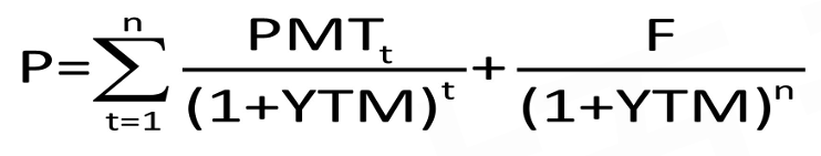
For option-free bonds
P=\sum_{t=1}^n \frac{P M T_t}{\left(1+Z_t\right)^t}+\frac{F}{\left(1+Z_n\right)^n}
Using spot rates that correspond to the maturities of the zero-coupon bonds to calculate the bond price
If market price is different with the calculated price, there is an arbitrage opportunity of "value additivity"
For bonds that have embedded options
The challenge one faces when developing a framework for valuing bonds with embedded options is that their expected future cash flows are depend on the change of interest rate
Changes in future interest rates impact the likelihood the option will be exercised and impact the cash flows
In order to develop a framework that values both bonds without and with embedded options, we must allow interest rates to take on different potential values in the future based on some assumed level of volatility
Term Structure Models
Modern Term Structure Models
Term structure models provide quantitatively precise descriptions of how interest rates evolve
Equilibrium term structure models: describe the dynamics of the term structure using fundamental economic variables that are assumed to affect interest rates
Cox-Ingersoll-Ross(CIR) model
Vasicek model
Arbitrage free models: assume bonds trading in the market are correctly priced (arbitrage free)
Ho-Lee model
Kalotay-Williams-Fabozzi (KWF) model
CIR Model
Higher interest rate → more investing → more capital supply → lower interest rate; and vice versa
Ultimately, interest rates will reach a market equilibrium rate at which no one needs to borrow or lend
Cox-Ingersoll-Ross (CIR) model is based on the idea that individuals must determine his optimal trade-off between consumption today and investing and consuming at a later time
\mathrm d {r}_{{t}}={k}\left(\theta-{r}_{{t}}\right) {\mathrm d t}+{\sigma} \sqrt{{r}_{{t}}} {\mathrm d Z}
\mathrm dr_t: a infinitely small change in short-term interest rate \mathrm dt: a infinitely small increase in time \theta: long-run value of the short-term interest rate r_t: the short-term interest rate k: a positive parameter for speed of mean reversion adjustment and the higher/lower, the quicker/slower \sigma: interest rate volatility \mathrm dZ: an infinitely small movement in a "random walk"
Drift term: {k}\left(\theta-{r}_{{t}}\right) {\mathrm d t}, which means the interest rate is mean-revert to long term value "0" with speed presented by parameter "k", also named deterministic term
Stochastic term: {\sigma} \sqrt{{r}_{{t}}} {\mathrm d Z}, also named volatility term. \sqrt{{r}_{{t}}} in the stochastic term tries to prevent interest rate to be non-negative, and assets that higher interest rate will lead to higher volatility
Vasicek model
\mathrm d {r}_{{t}}={k}\left(\theta-{r}_{{t}}\right) {\mathrm d t}+{\sigma} {\mathrm d Z}
Disadvantages of Vasicek model
Does not force interest rates to be non-negative
Volatility remains constant over the period of analysis
Ho-Lee model
\mathrm d {r}_{{t}}=\theta_t {\mathrm d t}+{\sigma} {\mathrm d Z}
The drift term, \theta_t, is time dependent, which means there is a value for \theta_t, at each time step
The Ho-Lee model, similar to the Vasicek model, has constant volatility, and interest rates may become negative
KWF Model
\mathrm d \ln{r}_{{t}}=\theta_t {\mathrm d t}+{\sigma} {\mathrm d Z}
The KWF model is analogous to the Ho-Lee model in that it assumes constant drift, no mean reversion, and constant volatility
KWF model describes the dynamics of the log of the short rate, and as a result, the log of the short rate is distributed normally, meaning the short rate itself is distributed lognormally.
The main implication of modeling the log of the short rate is that it will prevent negative rates
Binomial Tree Model
Binomial Interest Rate Tree
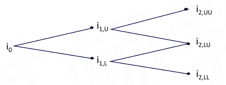
A interest rate model that assumes interest rates at any point of time(node) have an equal probability of taking one of two possible values in the next period, an upper path (U) and a lower path (L)
The binomial interest rate tree framework is a lognormal random walk(lognormal tree) that insures two appealing properties:
i_{1, U}=i_{1, L} \times e^{2\sigma} \quad i_{2, U U}=i_{2, L U} \times e^{2\sigma} \quad i_{2, U U}=i_{2, L L} \times e^{4\sigma}
Non-negativity of interest rates
higher volatility at higher interest rates
Estimation of volatility
Historical interest rate volatility: volatility is calculated by using data from the recent past with the assumption that what has happened recently is indicative of the future
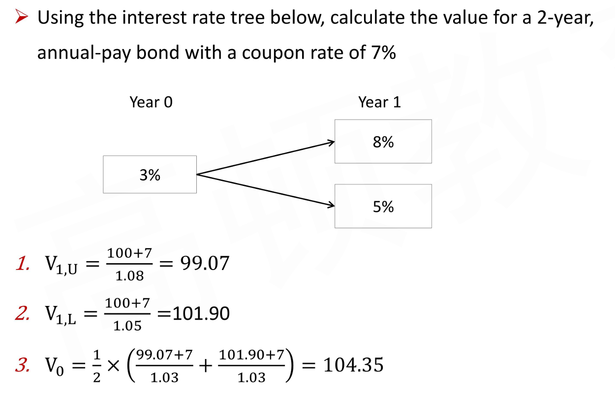
Value bond by moving backward from last period to time 0
Bond value at any node is the average PV of two possible values from next period
Discount rate is the one-period forward rate at that node
Example
Pathwise Valuation
For a binomial interest rate tree with n period, there will be 2^n paths
Calculate the present value of a bond for each possible interest rate path and takes the average of these values across paths
Monte Carlo Method
Binomial tree backward induction assumes cash flows are not path dependent, therefore it cannot value the securities with such cash flow.
Path dependency: cash flow to be received in a particular period depends on the path followed to reach its current level as well as the current level itself
Monte Carlo forward-rate simulation involves randomly generating a large number of interest rate paths, and it is often used when a security's cash flow are path dependent
For example, the valuation of MBS depends to a great extent on the level of prepayments, which are interest rate path dependent
Using the procedure just described, the model will produce benchmark bond values equal to the market prices only by chance
The constant added to all short interest rates is called a drift term
The model is said to be drift adjusted
Increasing the number of paths increases the accuracy of the estimate in a statistical sense
Yield curve modelers often include in the Monte Carlo estimation is mean reversion
We implement mean reversion by implementing upper and lower bounds on the random process generating future interest rates
Bonds with Embedded Options
Callable and Putable Bond
Bonds with Embedded Option
Basic Concepts
Callable Bond
Callable bonds give the issuer the option to call back the bond
Investor is long the straight bond but short the call option on the bond
At maturity, the holder of an extendible展期 bond has the right to keep the bond for a number of years after maturity, possibly with a different coupon
Putable and extendible bonds are equivalent
Convertible bond allows bondholders to convert their bonds into the issuer's common stock
Bonds with estate put allows the heirs继承人 of an investor to put the bond back to the issuer upon the death of the investor
The value of the estate put depends on the bondholder's life expectancy
The shorter the life expectancy, the greater the value of the estate put
Valuation by Binomial Interest Rate Tree
The basic process to value a bond with embedded option is similar to the valuation of straight bond
However, the following two points are different
Only binomial interest rate tree model is applicable, valuation with spot rates is non-available any more
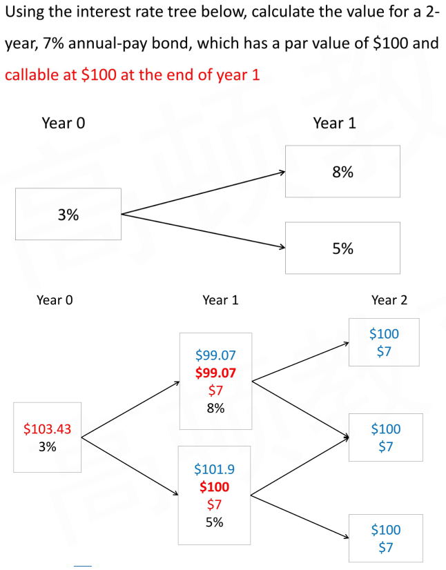
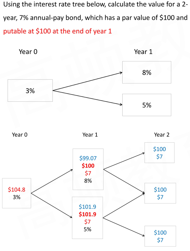
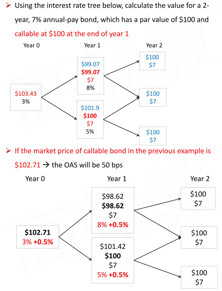
Need to check at each node to determine whether the embedded option will be exercised or not Call rule: the value of callable bond is the lower of the call price and the calculated price if the bond is not called Put rule: the value of putable bond is the higher of the put price and the calculated price if the bond is not put
Example of Callable Bond
Example of Putable Bond
Effects of Interest Rate Volatility
R_u=R_d \times e^{2\sigma \sqrt{t}}
R_d is the rate in the down state
\sigma is the interest rate volatility
t is the time in years between "time slices" (a year, so here t = 1)
Effects of Interest Rate Volatility
The value of a straight bond is unaffected by changes in the volatility of interest rate
Interest rate volatility affects the value of a callable or putable bond
The values of call and put options increase when interest rate volatility increases
As interest rate volatility increases, the value of the callable bond decreases
As interest rate volatility increases, the value of the putable bond increases
Option Adjusted Spread
Calculation of OAS
Option adjusted spread
yield spread that remove the influence of embedded option
When valuing risky bond with the interest rate tree generated from government spot curve, the model does not produce arbitrage-free price (typically higher than market price)
Option-adjusted spread(OAS) is the constant spread that, when added to all the one-period forward rates on the interest rate tree, makes the model price of the bond equal to its market price
OAS = Z-spread - Option value(%)
Callable bond → option value > 0 → OAS < Z-spread
Putable bond → option value < 0 → OAS > Z-spread
Example
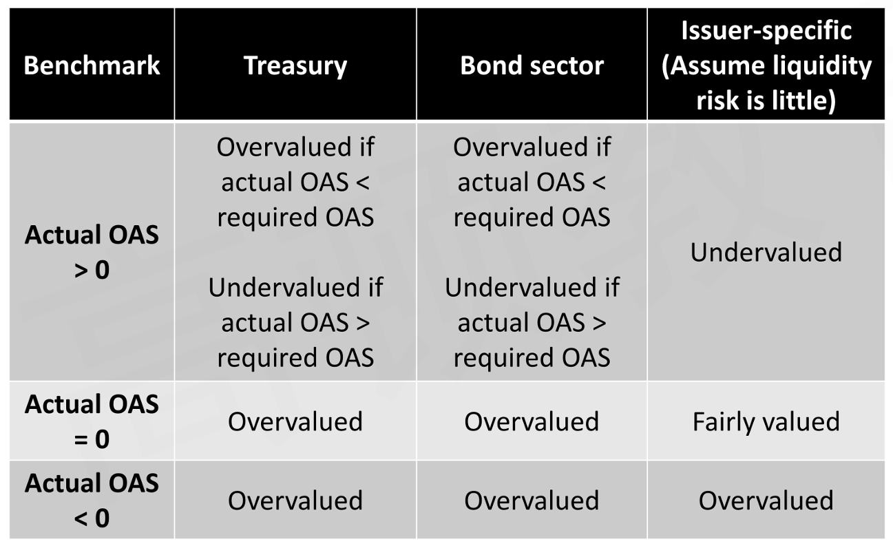
Application of OAS
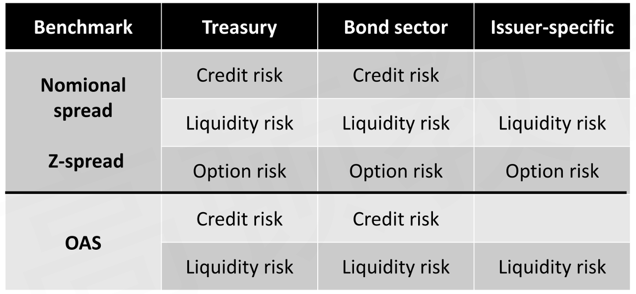
Comparison between Spreads
Option-Adjusted Spread
Interest Rate Volatility vs. OAS
The effect of volatility on the OAS for a bond embedded with option
As interest rate volatility increase, the OAS for the callable bond decreases
As interest rate volatility increase, the OAS for the putable bond increases
Interest Rate Risk
Effects of changes in the Shape of Yield Curve
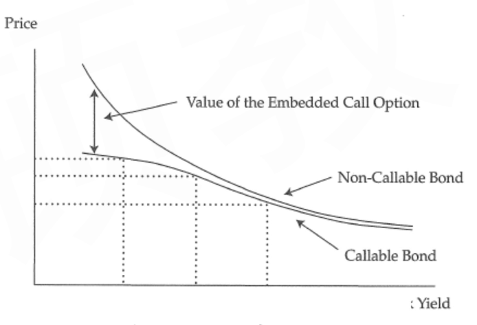
As interest rates decline, the value of the callable bond rises less rapidly than the value of the straight bond, limiting the upside potential for the investor
Call option value increases as interest rate decline
The rise of the straight bond value is partially offset by the increase in the value of the call option
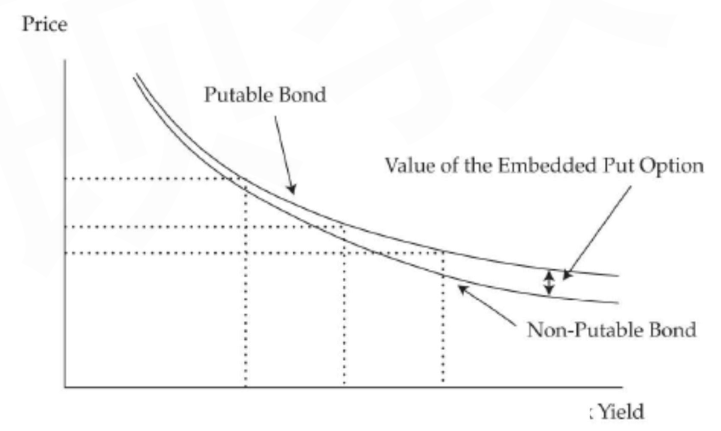
As interest rates rise, the value of the putable bond falls less rapidly than the value of the straight bond
Put option value increases as interest rates rise
The decline of the straight bond value is partially offset by the increase in the value of the put option
As the yield curve moves from being upward sloping, to flat, to downward sloping, the value of the call option increases
The one-period forward rates become lower and the opportunities to call increase
As the yield curve moves from being upward sloping, to flat, to downward sloping, the value of the put option decreases
The one-period forward rates become lower and the opportunities to put declines
Effective Duration
In the presence of embedded options, we use the binomial model to compute effective duration, and the process to calculate the PV_- and PV_+, is as following:
calculate the implied OAS to the current binomial tree according to the market price (PV_0)
shift the benchmark yield curve down by ,generate a new interest rate tree, and then calculate the PV_- using the OAS calculated in step 1
shift the benchmark yield curve up by , and calculate the PV_+. with similar method
calculate the bond's effective duration using the formula
Properties of Effective Duration
ED of zero-coupon bond ≈ maturity of the zero-coupon bond
ED of fixed-rate bond < maturity of the fixed-rate bond
ED of floating-rate bond ≈ time (years) to next reset
ED of both callable and putable bond ≤ ED of of identical straight bond
Decrease of interest rate will decrease the effective duration of callable bond
Increase of interest rate will decrease the effective duration of putable bond
Effective Convexity
Straight bond
Always exhibits low positive convexity
The increase in the value of an option-free bond is higher when rates fall than the decrease in value when rates increase by an equal amount
Callable bond
When interest rates are high, callable and straight bond have similar positive convexity
When the call option is in the money, the effective convexity of the callable bond turns negative
Putable bond
Always have positive convexity
When the put option is in the money, the effective convexity of the putable bond is higher than straight bond
One-Sided Duration
One-sided durations are the effective durations when interest rate curves go up or down
One-sided durations are better at capturing the interest rate sensitivity of a callable or putable bond than the(two-side)effective duration, particularly when the embedded option is near the money
One-side up-duration: durations that apply only when interest rate curve rises
One-side down-duration: durations that apply only when interest rate curve falls
Key Rate Duration
Definition of Key Rate Duration
Key rate durations measure the sensitivity of the bond's price to changes in specific maturities on the benchmark yield curve
Shifting any par rate has an effect on the value of the bond
Key rate durations help to identify the "shaping risk" for bonds Shaping risk: the sensitivity of bond's price to changes in the shape of the yield curve (e.g., steepening and flattening)
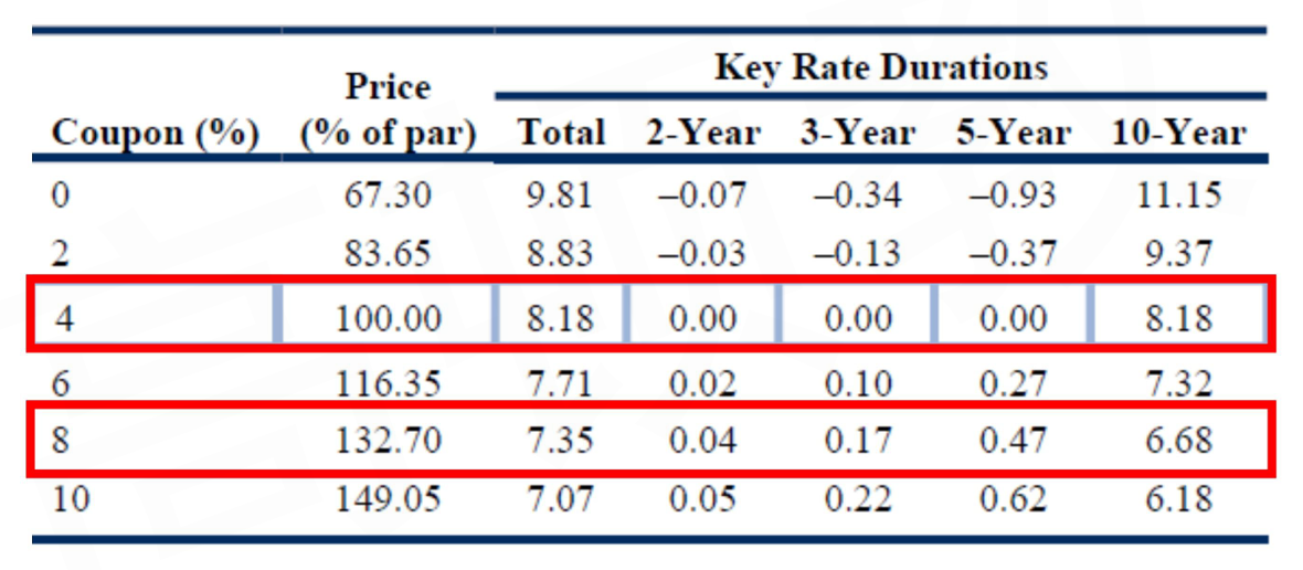
For option-free bond that is traded at par
Bond's maturity matched rate is the only rate that affects the bond's value
All other key rate durations are zero
For option-free bond that is not traded at par
Shift the maturity-matched par rate has the greatest effect
Example for Key Rate Durations of 10-Year Option-Free Bonds Valued at a 4% Flat Yield Curve
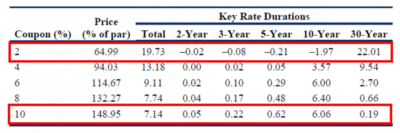
For callable bonds
With low coupon rate
The callable bonds are unlikely to be called
The rate that has the highest effect on the value of the callable bond is the maturity-matched rate
As the bond's coupon increase
So does the likelihood of the bond being called
The rate that has the highest effect on the callable bond value is the time-to-exercise rate
Example for Key Rate Durations of 30-Year Bonds Callable in 10Years Valued at a 4% Flat Yield Curve with 15% Interest Rate Volatility
For putable bonds
With high coupon rate
The putable bonds are unlikely to be put
Prices are most sensitive to their maturity-matched rates
As the bond's coupon decrease
So does the likelihood of the bond being put
price is most sensitive to the time-to-exercise rate
For zero-coupon bond or bond with a verylow coupon
Key rate durations can sometimes be negative for maturity points that are shorter than the maturity of the bond being analyzed
Capped or Floored Floating-Rate Bond
Definition and Application
Floating-Rate Bonds(Floaters)
The coupon rate is linked to an external reference rate, such as LIBOR
Coupon rate = reference rate + quoted margin
Reference rate reset periodically, typically quarterly
Quoted margin is usually constant
Coupon payments are in arrears: based on previous period's reference rate
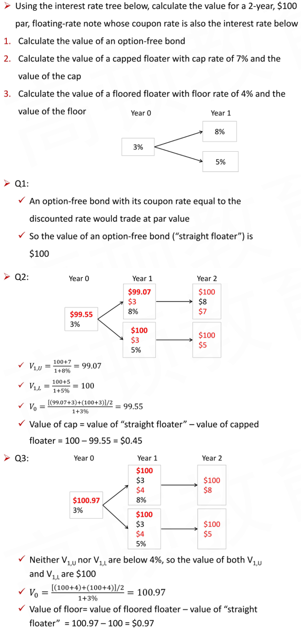
Floater with Cap or Floor
Capped floating-rate bonds'coupon rate would not exceed the specified maximum rate (cap)
Floored floating-rate bonds' coupon rate would not fall below the specified minimum rate (floor)
A capped floaterprotects the issuer against rising interest rates and is thus an issuer option
The investor is long the bond but short the embedded "cap" option
Value of capped floating-rate bond = value of a "straight" floater - value of the embedded cap
Calculation of Floater with Cap or Floor
Similarly, capped and floored floaters can be valued by using the backward induction method in a binomial interest rate tree
We check whether the cap or floor applies at each node
If it does, the cash flow is adjusted accordingly
Example
Ratchet Bond
As with conventional floater, ratchet bond's coupon is reset periodically according to a formula based on a reference rate and a credit spread
Ratchet bonds are floating-rate bonds with both issuer and investor options
Ratchet bonds offer extreme protection as a capped floater protects the issuer against rising interest rates
At the time of reset, the coupon can only decline: it can never exceed the existing level
So, over time, the coupon "ratchets down"
At issuance, the coupon of a ratchet bond is much higher than that of a standard floater
Whenever a coupon is reset, the investor has the right to put the bonds back to the issuer at par
The embedded option is called a "contingent put", because the right to put is available to the investor only if the coupon is reset
Convertible Bond
Basic Concepts of Convertible Bond
Conversion ratio: the number of common shares that the bondholder receives from converting the bonds into shares
Conversion price = Issue price/ Conversion ratio
Typically, conversion bonds are issued at par value
Conversion ratio = Issue price/ Conversion price
Market conversion price: the price that investors effectively pay for the underlying common share if they buy the convertible bond and then convert it into shares
Market conversion price = Convertible bond price/ Conversion ratio
Market conversion premium ratio = Market conversion premium per share / Market share price
Conversion value: the value of the bond if it is converted to common shares
Conversion value = Market share price x Conversion ratio
Conversion ratio is fixed but the market share price is floating, so the conversion value is floating
Straight value: the value of the bond if it were not convertible
The PV of the cash flows
Minimum value is a floor value for the convertible bond at the greater of the conversion value or the straight value
Minimum value = Max(conversion value, straight value)
Analysis of Convertible Bond
Risk-Return Characteristics of Convertible Bond
Downside risk
Straight value can be used as a benchmark of the downside risk of a convertible bond Premium over straight value =(Convertible bond price / Straight price) - 1
Upside potential
Depends primarily on the prospects of the underlying common share
Influence of stock price
Stock price increases
Convertible bond will underperform
Reason: conversion premium
Stock price decreases
Returns on convertible bonds exceed those of the stock
Reason: The convertible bond's price has a floor value
Stock price remains stable
Returns on convertible bonds exceed those of the stock
Reason: The coupon payments received from the bond, assuming no change in interest rates or credit risk of the issuer
When the underlying share price is well below the conversion price, the convertible bond exhibits mostly bond risk-return characteristics
Straight value acts as a downside limit
Price of the common stock has little or no effect on the convertible's market price
When the underlying share price is well above the conversion price, the convertible bond exhibits mostly stock risk-return characteristics
In between these two extremes, the convertible bond trades like a hybrid instrument
Valuation Equivalence
The convertible bond can be valued as the equivalence of its component combination
Convertible bond = Straight bond + Call option on stock
Credit Analysis Models
Modeling Credit Risk
Loss Given Default
Expected loss = Probability of default x Loss given default
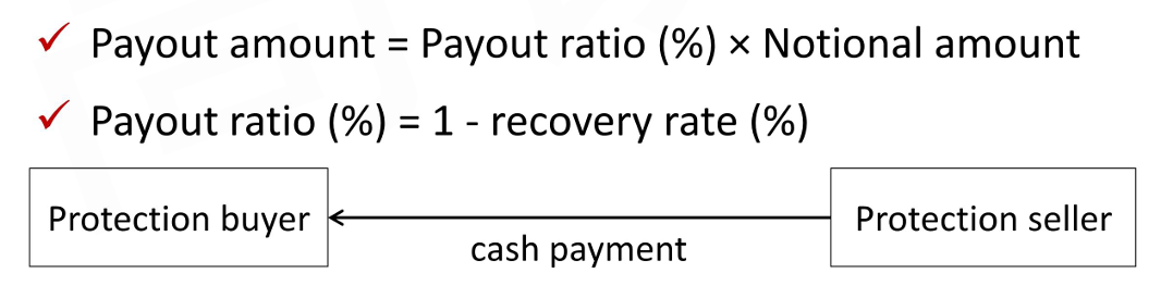
Loss given default(LGD) is the amount of loss if a default occurs
Loss given default(%) = 100% - Recovery rate
Loss given default($) = Expected exposure - Recovery($)
Recovery rate is percentage of the loss recovered from a bond in default
Expected exposure is the projected amount of money the investor could lose if an event of default occurs, before factoring in possible recovery
Probability of Default
Expected loss = Probability of default x Loss given default
Probability of default (POD) is the probability that the bond issuer will not meet its contractual obligations on schedule
Actual probability of default
The actual default probability for the corporate bond can observed from historical data
Risk-neutral probability of default
"Risk-neutral" follows the usage of the term in option pricing
In the risk-neutral option pricing methodology, the expected value for the payoffs is discounted using the risk-free interest rate
Usually, risk-neutral default probability is higher than actual default probability
The observed spread over the yield on a risk-free bond in practice also includes liquidity and tax considerations in addition to credit risk
The initial POD, which is called the hazard rate in statistics, is used to calculate the remaining PODs
Hazard rate is the conditional default rate, which means the default rate under the condition that no default happens before
Probability of survival(POS) is under the condition that no default happens before
Credit Valuation Adjustment
Fair value of corporate bond = VND - CVA
VND: the value for the corporate bond assuming no default
Credit valuation adjustment(CVA) is the value of the credit risk in present value term
CVA is the sum of PV of expected loss
Credit Spreads
Components of a Corporate Bond Yield
Benchmark Yield capture the macroeconomic factors affecting all debt securities
Expected real rate of return
Expected inflation rate
Risk aversion: compensation for uncertainty regarding expected inflation
Spread Over the Benchmark Yield capture the microeconomic factors that pertain to the corporate issuer and the specific issue itself
Expected loss from default
Liquidity
Taxation
Risk aversion: compensation for uncertainty regarding expected loss from default
Term Structure of Credit Spreads
Term structure of credit spreads is the curve that shows the spread over a benchmark security for an issuer for outstanding fixed-income securities with shorter to longer maturities
When a bond is very likely to default, it often trades close to its recovery value at various maturities
The credit spread curve is less informative about the relationship between credit risk and maturity
Key Drivers of the Term Structure of Credit Spreads
Credit quality
The credit term structure for highly rated securities tends to be either flat or slightly upward sloping
Securities with lower credit quality face greater sensitivity to the credit cycle
It results in a steeper credit spread curve or sometimes face a downward-sloping credit term structure
Financial conditions
A stronger economic climate is generally associated with lower credit spreads for issuers whose default probability declines
Market supply and demand dynamics
The credit curve will be most heavily influenced by the new and most frequently traded securities
Infrequently traded bonds trading with wider bid-offer spreads can also impact the shape of the term structure
Company-value model
These models take stock market valuation, equity volatility, and balance sheet information into account to derive the implied default probability for a company
For example, greater equity volatility will tend to drive a steeper credit spread curve
Appropriate risk-free or benchmark rates used to determine spreads
The duration and maturity of the most liquid or on-the-run government bonds rarely match that of corporate, so it is often necessary to interpolate
As the interpolation may impact the analysis for less-liquid maturities, the benchmark swap curve based on interbank rates is often substituted for the government
Term structure analysis should include only bonds with similar credit characteristics, which are typically senior unsecured general obligations of the issuer
Any bonds of the issuer with embedded options, first or second lien provisions, or other unique provisions should be excluded from the analysis
Sometimes securities typically include cross-default provisions,so that all securities across the maturity spectrum of a single issuer will be subject to recovery in the event of bankruptcy
Credit Analysis for Securitized Debt
ABS vs. Corporate Debt
In the case of a corporate bond, when the issuer defaults, the cash flows cease and there is a terminal cash flow
ABS do not default, but they can lose value as the SPE's pool of securitized assets incurs defaults
The credit risk metric of probability of loss is applied rather than probability of default
Credit Analysis for Securitized Debt
Granularity of the portfolio
A highly granular portfolio may have hundreds of underlying creditors, suggesting it is appropriate to draw conclusions about creditworthiness based on portfolio summary statistics rather than investigating each borrower
Alternatively, an asset pool with fewer discrete or non-granular investments would warrant analysis of each individual obligation
Homogeneity
Analyst might draw general conclusions about the nature of homogeneous obligations (eg. credit card or auto loan) given that an individual obligation faces strict eligibility criteria to be included in a specific asset pool
Heterogeneous leveraged loan, project finance, or real estate transactions require scrutiny on a loan-by-loan basis given their different characteristics
Investors are exposed to the ability of the servicer to effectively manage and service the portfolio over the life of the transaction
Structure of a collateralized or secured debt transaction is a critical factor in analyzing securitized debt
Bankruptcy remoteness can separate risk between the originator and SPE
Additional credit enhancements are a key structural element to be evaluated in the context of credit risk
Credit Analysis for Covered Bond
A covered bond is a senior debt obligation of a financial institution that gives recourse to the originator/issuer as well as a predetermined underlying collateral pool
The dual recourse双重还款源 to both the issuing financial institution as well as the underlying asset pool has been a hallmark of covered bonds
Credit Models
Credit Scores and Credit Ratings
Credit scoring ranks a borrower's credit riskiness
Provide an ordinal ranking of a borrower's credit risk
Do not tell the degree to which the credit risk differs among different ranks
Used for small businesses and individuals
The FICO(Fair Isaac Corporation) score is used in the United States by about 90% of lenders to retail customers
Five primary factors are included in the proprietary algorithm used to get the score:
35% for the payment history
30% for the debt burden
15% for the length of credit history
10% for the types of credit used
10% for recent searches for credit
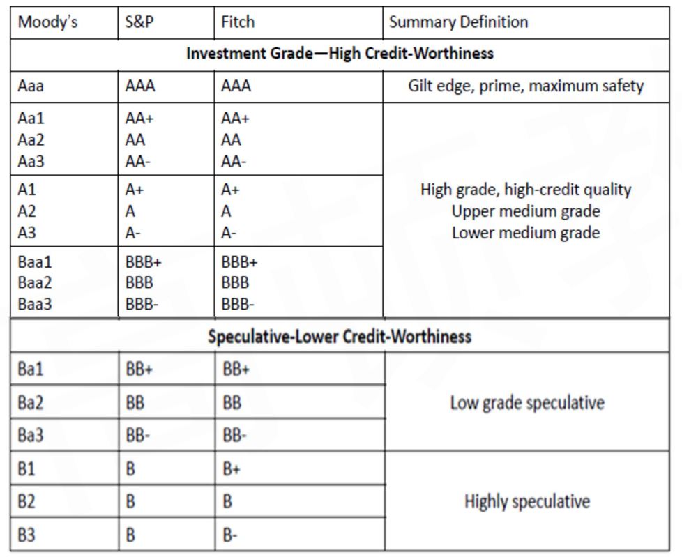
Credit ratings rank the credit risk of a company, government(sovereign),quasi-government,or ABS
Strengths of credit ratings
Provide a simple statistic
Tend to be stable over time, reducing debt market volatility
Weaknesses of credit ratings
The stability reduces the correspondence to a debt's default probability, and make the rating lag the market
Do not depend on business cycle, while default probability does
The issuer-pays model for compensating credit-rating agencies has a potential conflict of interest that may distort the accuracy of credit ratings
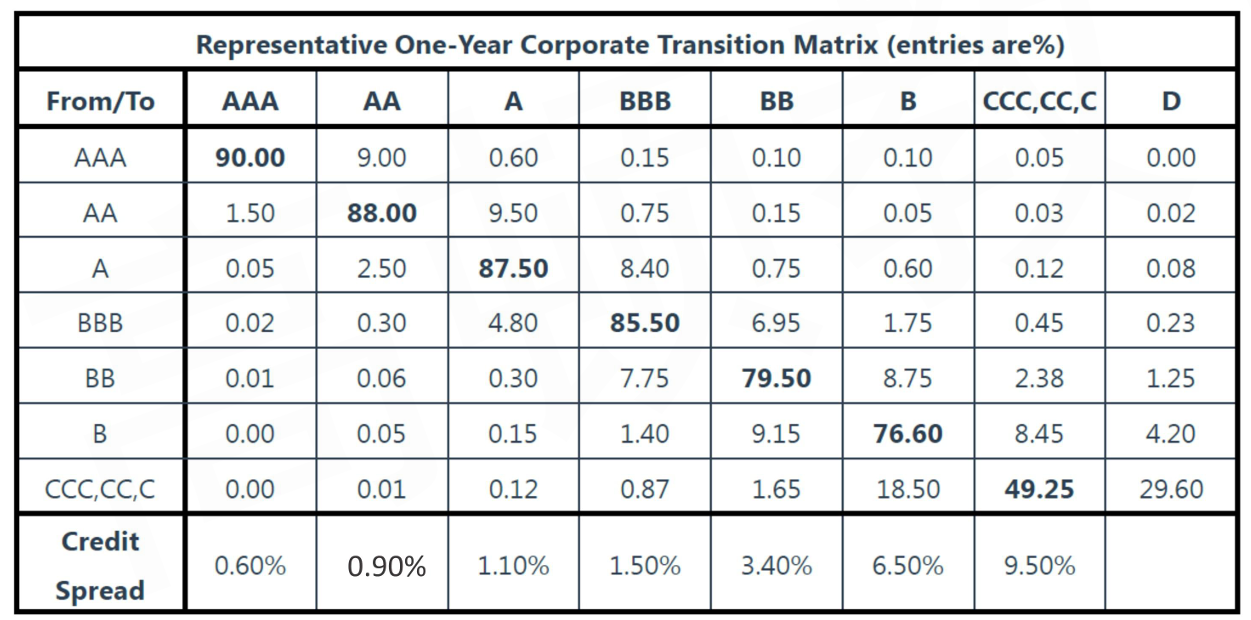
Credit Transition Matrix
Credit transition matrix shows the probabilities of a particular rating transitioning to another over the course of the following year
Structural Model
Assumptions of structural models
Company's assets(A) are traded in a frictionless arbitrage-free market
The company has a simple balance sheet structure with only one class of simple zero-coupon debtD(K,t)
The value of the company's assets has a lognormal distribution
The risk-free interest rate (r) is constant over time
The probability of default is endogenous内生的 (internal) to this structural model
Call Option Analogy
E_t=\max \left(A_t-K,0\right) Company's equity is economically equivalent to owning a European call option on the company's assets (A_t) with strike price K (face value of zero-coupon debt) and maturity t (maturity of debt)
D_t=A_t-\max \left(A_t-K,0\right)
Company's debt is economically equivalent to owning the company asset, and simultaneously selling a European call option on the assets (A_t) of the company with strike price K (face value of zero coupon debt) and maturity t
Put Option Analogy
D_t=K-\max \left(K-A_t,0\right)
Company's debt is economically equivalent to owning a riskless bond, and simultaneously selling a European put option on the assets (A_t) of the company with strike price K(face value of zero-coupon debt) and maturity t
Option Analogy for Debt
owning the company asset, and simultaneously selling a European call option on the assets
owning a riskless bond, and simultaneously selling a European put option on the assets
Strengths
It provides insight into the nature of credit risk
The company defaults when the value of its assets fall below the default barrier
Provide an option analogy for understanding a company's default probability and recovery rate
Can be estimated using only current market prices
Weaknesses
Model assumptions of simple balance sheet and traded assets are not realistic
Estimation procedures do not consider business cycle
Reduced-Form Model
Assumptions of reduced-form models
The company's zero-coupon bond trades in frictionless markets that are arbitrage free
Risk-free interest rate (r) is stochastic随机变量
Economy and recovery rate are stochastic
Probability of default is not constant and varies with the state of economy
Reduced-form models treating default as an exogenous (external) variable that occurs randomly
Under reduced form models, debt value can be computed as:
D_t=\tilde{E}\left(\frac{K}{\prod\left(1+r_i\right)}\right)
Strengths
Model inputs are observable, historical estimation procedures can be used
Credit risk allowed to fluctuate with business cycle
Do not require specification of the company's BS structure
Weaknesses
Do not explain the economic reasons for default
Unless the model has been formulated and back tested properly, the hazard rate estimation may not be valid
Credit Default Swaps
Structure and Features of CDS
Credit Derivative
Credit derivative is a derivative instrument in which the underlying is the credit quality of a borrower
Four types of credit derivative
Total return swaps
Credit spread options
Credit-linked notes
Credit default swaps(CDS)
Definition of CDS
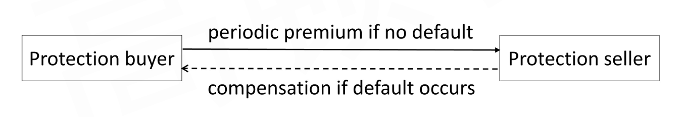
Credit default swaps (CDS) is a derivative contract between two parties, credit protection buyer and credit protection seller, in which the buyer makes a series of cash payments to the seller and receives a promise of compensation for credit losses resulting from the default (a pre-defined credit event) of a third party
Protection buyer / CDS buyer is the one who short CDS
Protection seller/ CDS seller is the one who long CDS
Fundamentals of CDS
CDS is essentially an insurance contract
Notional amount/principal保额 is the amount of protection being purchased
CDS spread(%)保费 is the premium that the buyer of a CDS pays to the seller for protection against credit risk
CDS spread is either paid upfront or over a period of time
Pricing of CDS Spread
The higher the probability of default, the higher the CDS spread
The higher the loss given default, the higher the CDS spread
Credit Events
Bankruptcy: allows the defaulting party to work with creditors under the supervision of the court so as to avoid full liquidation
Failure to pay: a borrower does not make a scheduled payment of principal or interest on any outstanding obligations after a grace period, without a formal bankruptcy filing
Restructuring: the issuer forces its creditors to accept terms that are different than those specified in the original issue.
Reduction or deferral of principal or interest
Change in seniority or priority of an obligation
Change in the currency in which principal or interest is scheduled to be paid
Settlement Protocols
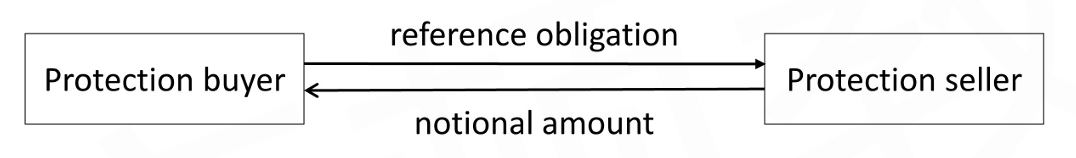
Physical settlement: actual delivery of the debt instrument in exchange for a payment by the credit protection seller of the notional amount of the contract
Cash settlement: the credit protection seller pays cash to the credit protection buyer
Types of CDS
Single-Name CDS
Single-name CDS is a CDS on one specific borrower(reference entity)
Reference obligation is a particular debt instrument issued by the borrower that is the designated instrument being covered by CDS
The designated instrument is usually a senior unsecured obligation, but the reference obligation is not the only instrument covered by the CDS
Any debt obligation issued by the borrower that is pari passu(ranked equivalently in priority of claims) or higher relative to the reference obligation is covered
The payoff of the single-name CDS is determined by the cheapest-to-deliver obligation
Cheapest-to-deliver obligation is the debt instrument that can be purchased and delivered at the lowest cost but has the same or higher seniority as the reference obligation
Index CDS
Index CDS(CDX) is a CDS that allows participants to take positions on the credit risk of a combination of borrowers
The notional principle is the sum of the protection on all the borrowers
Credit correlation is a key determinant of the value of an index CDS
The more correlated the defaults, the more costly it is to purchase protection for a combination of the companies
Pricing of CDS
CDS Spread and Fixed Coupon
CDS spread(%) is the premium that the buyer of a CDS pays to the seller for protection against credit risk
Standardization in the market has led to a fixed coupon (CDS coupon rate) on CDS 1% for a CDS on an investment-grade company or index 5% for a CDS on a high-yield company or index
Upfront Payment
Upfront payment ($) = Total present values of protection leg - Total present values of premium leg
Premium leg: The series of payments the credit protection buyer promises to make to the credit protection seller
Protection leg: The contingent payment that the credit protection seller may have to make to the credit protection buyer
Upfront Premium
Upfront premium is the differential between the credit spread and the standard fixed coupon rate that converted to a present value basis
A credit spread more than the standard coupon rate will result in a cash upfront payment from the protection buyer to the seller
A credit spread less than the standard rate would result in a cash upfront payment from the protection seller to buyer
Upfront premium(%) ≈ (Credit spread - Fixed coupon) × Duration
Upfront premium (%) ≈ Total present values of credit spread - Total present values of fixed coupon
Credit spread ≈ Upfront premium / Duration + Fixed coupon
CDS Pricing Conventions
Price of CDS in currency per 100 par ≈ 100 - upfront premium(%)
Upfront premium(%)= 100 -Price of CDS in currency per 100 par
Profits of CDS
The value of a CDS may change if the credit quality of the reference entity or the credit risk premium in the overall market change
Monetizing a gain or loss: changes in the value of a CDS gives rise to opportunities to unwind the position
Profit(%) ≈ Change in spread(%) × Duration of CDS
Profit($) ≈ Change in spread(%) × Duration of CDS × Notional amount($)
Applications of CDS
A derivative instrument has two general uses
One is to exploit an expected movement in the underlying Managing credit exposure: Taking on or shedding of credit risk
The other trading opportunity is in valuation differences between the derivative and the underlying Valuation disparity: The focus is on differences in the pricing of credit risk in the CDS market relative to that of the underlying bonds
Managing Credit Exposure
Adjustment of credit exposure: increasing/decreasing credit exposure by selling/buying CDS if having assumed too little/much credit risk
Naked CDS: buying or selling credit protection without credit exposure to the reference entity
The buyer (seller) of a naked CDS is taking a position that the entity's credit quality will deteriorate (improve)
Long/short trade: taking a long position in one CDS and a short position in another
A bet that the credit position of one entity will improve relative to that of another
Managing Credit Exposure
Credit curve is the credit spreads for a range of maturities of a company's debt Upward-sloping credit curves imply a greater likelihood of default in later years, which are more common than downward-sloping curves
Curve trade: buying a CDS of one maturity and selling a CDS on the same reference entity with a different maturity
If an investor believes that the credit curve will become steeper, he can buy a long-term CDS and sell a short-term CDS
If an investor believes that the credit curve will become flatter,he can buy a short-term CDS and sell a long-term CDS
Valuation Disparity
Basis trade: exploit the difference of credit spread between bond market and CDS market
In principle, the amount of yield attributable to credit risk on the bond should be the same as the credit spread on a CDS
The general idea behind is that any such mispricing will disappear when the market recognizes the disparity
Another type of trade using CDS can occur within the instruments issued by a single entity
Arbitrage trade: buy the cheaper and sell the more expensive
If the cost of the index is not equivalent to the aggregate cost of the index components
If a synthetic CDO is not equivalent to the actual CDO Synthetic CDO is created by combining a portfolio of default-free securities with a combination of credit default swaps undertaken as protection sellers

 i_{1, U}=i_{1, L} \times e^{2\sigma} \quad i_{2, U U}=i_{2, L U} \times e^{2\sigma} \quad i_{2, U U}=i_{2, L L} \times e^{4\sigma}