Determining the value of an asset is at the heart of analysts professional activities and skill in valuation is a very important element of success in investing
Valuation is the estimation of an asset's value based on:
Variables perceived to be related to future investment returns
Or, on comparisons with similar assets
Or, on estimates of immediate liquidation proceeds
Intrinsic value is the value of the asset given a hypothetically complete understanding完全掌握资产的所有信息下的估值 of the asset's investment characteristics
Sources of Perceived Mispricing
There are two sources of perceived mispricing(V_E-P)
E(IV)-P=(IV-P)+(E(IV)-IV)
IV-P: true mispricing
E(IV)-IV: estimation error
The difference between the true (real) but unobservable intrinsic value and the observed market price contributes to the abnormal return or alpha which is the concern of active investment managers
Other Definitions of Value / Price
Fair market value (price) is the price at which a willing, informed, and able seller would trade an asset to a willing, informed, and able buyer
Investment value is the value to a specific buyer taking account of potential synergies and based on the investor's requirements and expectations
Intrinsic value is most relevant to public company valuation
Going-Concern and Liquidation
Going-concern value
The value under a going-concern持续经营 assumption that the company will continue its business activities into the foreseeable future
Liquidation value
The value if the company is dissolved and its assets sold individually
Orderly liquidation value assumes adequate time to realize liquidation value
Going-concern value > Liquidation value
Valuation Model Selecting
Valuation Models
Absolute valuation models
Models that specify an asset's intrinsic value which is in order to be compared with the asset's market price
It does not need consider about the value of other firms
Relative valuation models
Models that derive values from relative comparison to similar assets,based on law of one price
It is typically implemented using price multiples
For examples P/E_{stock} \lt P/E_{market} → stock is relatively undervalued
Models Selection
Consistent with characteristics of company
Understand the company and how its assets create value
Based on quality and availability of data
DDM problematic when no dividends
P/E problematic with highly volatile earnings
Consistent with purpose of analysis
Free cash flow vs. dividends for controlling interest
Common Adjustments for Valuation
The value of a stock investment that would give an investor a controlling position will generally reflect a control premium
The value of non-publicly traded stocks generally reflects a lack of marketability discount
Among publicly traded(i.e., marketable) stocks, the prices of shares with less depth to their markets (less liquidity) often reflect an illiquidity discount
The price that could be realized for that block of shares would generally be lower than the market price for a smaller amount of stock, a so-called blockage factor
Sum-of-the-Parts Value
Sum-of-the-parts value (breakup value, private market value) is the value for a company as a whole obtained by adding up the values of individual parts of the firm
Useful when valuing a company with segments in different industries that have different valuation characteristics
Frequently used to evaluate the value that might be unlocked in a restructuring through a spinoff, split-off, or equity (IPO) carve-out
Conglomerate Discount
Conglomerate discount多元化经营折价 refers to the concept that the market applies a discount to the stock of a company operating in multiple, unrelated businesses compared to the stock of companies with narrower focuses
Possible explanations for the conglomerate discount include:
Inefficiency of internal capital markets
Companies' allocation of investment capital among divisions does not maximize overall shareholder value
Endogenous factors
Poorly performing companies tend to expand by making acquisitions in unrelated businesses
Research measurement errors
Process of Valuation
Steps of Valuation Process
Understanding the business
Industry and competitive analysis
Analysis of financial reports
Considerations in using accounting information
Forecasting company performance
A top-down forecasting approach moves from international and national macroeconomic forecasts to industry forecasts and then to individual company and asset forecasts
A bottom-up forecasting approach aggregates forecasts at a micro level to larger scale forecasts
Selecting the appropriate valuation model
Converting forecasts to a valuation
Applying the valuation conclusion
Sell-side analysts associated with investment firms' brokerage operations are perhaps the most visible group of analysts offering valuation judgments
Buy-side analysts works in investment management firms,trusts and bank trust departments, and similar institutions, an analyst may report valuation judgments to a portfolio manager or to an investment committee as input to an investment decision
Applications of Equity Valuation
Selecting stocks
Inferring (extracting) market expectations
Evaluating corporate events
Rendering fairness opinions
Evaluating business strategies and models
Communicating with analysts and shareholders
Appraising private businesses
Share-based payment (compensation)
Contents of a Research Report
Contain timely information
Be written in clear, incisive language
Be objective and well researched, with key assumptions clearly identified
Distinguish clearly between facts and opinions
Present sufficient information to allow a reader to critique the valuation
State the key risk factors involved in an investment in the company
Disclose any potential conflicts of interests faced by the analyst
Discounted Dividend Valuation
Framework of Model
Models
DCF Model
{V}_0=\sum_{{i}=1}^{+\infty} \frac{{CF}_{{i}}}{(1+{r})^{{i}}}
An asset's intrinsic value is the present value of its expected future'cash flows'
DDM Model
V_0=\sum_{i=1}^{+\infty} \frac{D_i}{\left(1+r_e\right)^i}
DDM shows the intrinsic value to the investor is the present value of all future dividends discounted at required return of equity
DDM is from the perspective of non-controlling investors'judgment of stock's intrinsic value
Advantages and disadvantages of DDM
Infinite Stream
Forecast the stock price at a certain point in the future
V_0=\sum\frac{D_i}{(1+r)^i}+\frac{P_n}{(1+r)^n}
Future dividends can be forecast by assuming one of several stylized growth patterns
Constant growth forever(Gordon growth model)
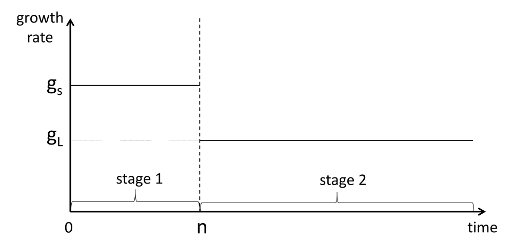
Two distinct stages of growth
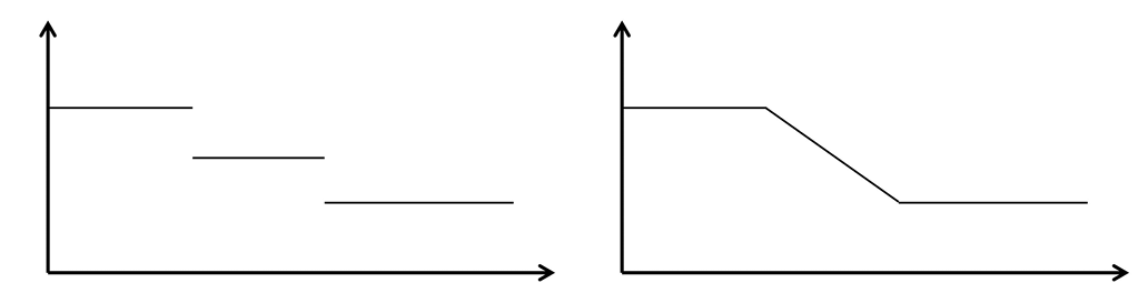
Three (or more) distinct stages of growth
A finite number of dividends can be forecast individually up to a terminal point, then the terminal value is estimated
Forecasted value at beginning of the final mature growth phase
The terminal value is then discounted back, and added to the present value of prior stage dividends
Two methods are often used
Apply a price multiple to a projected terminal value of a fundamental such as P/E, P/B
Gordon growth model
Gordon Growth Model
Basic Concepts of GGM
Gordon Growth Mode
V_0=\frac{D_1}{r_e-g}
Assumptions of Gordon Growth Model
Dividends grow at constant rate (g) forever
Growth rate is less than required return (r_e \gt g)
Considerations of Using Gordon Growth Model
The GGM should reflect long-term growth expectations: GDP growth, industry life cycle stages and the impact of the five force model
The model's intrinsic values V_0 are very sensitive to the input variables for r_e and g Sensitivity analysis may be required to obtain a range of values rather than a specific point estimate of value
Gordon growth model can accurately value companies that are repurchasing shares when the analyst can appropriately adjust the dividend growth rate for the impact of share repurchases
Sustainable Growth Rate
SGR(g) is the sustainable growth rate in earnings and dividends if we assume:
Growth from internally generated sources (No new equity issued)
Some key financial ratios remain unchanged
SGR(g)= ROE × retention rate(b)
ROE is calculated using beginning-of-period shareholders' equity
The lower the earnings retention ratio, the lower the growth rate(dividend displacement of earnings)
PRAT model: SGR = Net Profit Margin × Total Asset Turnover × Financial Leverage × retention rate
Applications of GGM
Valuation of Preferred Stock
V_0=\frac{D_p}{r_p}
The discount rate or capitalization rate is often at a positive spread over the firms junior ranking debt yield
Justified P/E Ratio
The Gordon model can also be used to calculate a "justified (or fundamental)"price multiple
Justified leading P/E Ratio
\text{Justified leading P/E}=\frac{V_0}{E_1}=\frac{\frac{D_1}{r-g}}{E_1}=\frac{\frac{D_1}{E_1}}{r-g}=\frac{1-b}{r-g}
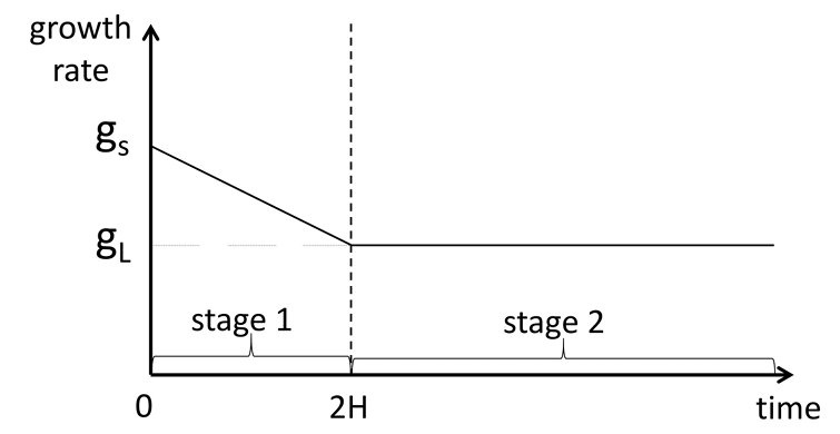
High growth followed by linearly declining followed by perpetual growth
Strengths
Ability to model many growth patterns
Solve for V, implied g, and implied r
Weaknesses
Require high-quality inputs (GIGO)
Model must be fully understood
Value estimates are sensitive to g and r
Model suitability is very important
Spreadsheet Modeling
In practice we can use spreadsheets to model any pattern of dividend growth
It can involve a great deal of information and can project different growth rates for differing periods
The reason for this is the inherent flexibility and computational accuracy of spreadsheet modeling.
Free Cash Flow Valuation
Basic Concepts of FCFs
Introduction of Free Cash Flows
Dividends are the cash flows actually paid to stockholders
Free cash flows(FCF) are the cash flows available for distribution after:
Fulfilling all obligations (operating expenses and taxes)
Without impacting on the future growth plans of the company (incremental working capital and fixed capital)
Strengths of FCFs
Used with firms that have no dividends
Functional model for assessing alternative financing policies
Rich framework provides additional detailed insights into company
Other measures such as EBIT, EBITDA, and CFO either double count or omit important cash flows
Limitations of FCFs
FCF may be negative due to large capital demands
Requires detailed understanding of accounting and FSA
Information may be not readily available or published
Free Cash Flows vs. Dividends
The logics behind the general valuation models are the same for both DDM and FCF models, but the numerator is different
FCFE could be either greater or less than dividends, but the same economic forces that lead to low (high) dividends lead to low (high) FCFE
Ownership perspective is very different between DDM and FCF model
FCFE model takes a control perspective and can be used in control perspective
DDM takes a minority perspective and can be used in valuing minority position in publicly traded shares
FCFF and FCFE
FCFF is the cash available to shareholders and bondholders after taxes,capital investment, and WC investment, pre-levered cash flow
FCFE is the cash available to equity holders after payments to and inflows from bondholders, post-leveraged cash flow
The two FCF approaches, indirect and direct, for valuing equity should theoretically yield the same estimates, if all inputs reflect identical assumptions
An analyst may prefer to use one approach rather than the other because of the characteristics of the company being valued
If the company's capital structure is relatively stable, using FCFE to value equity is more direct and simpler
The FCFF model is often chosen in two other cases:
Alevered company with negative FCFE
Alevered company with a changing capital structure
Calculations of FCFs
Calculating FCFF
Basic Formula
FCFF=EBIT\times(1-t)+NCC-WCInv-FCInv
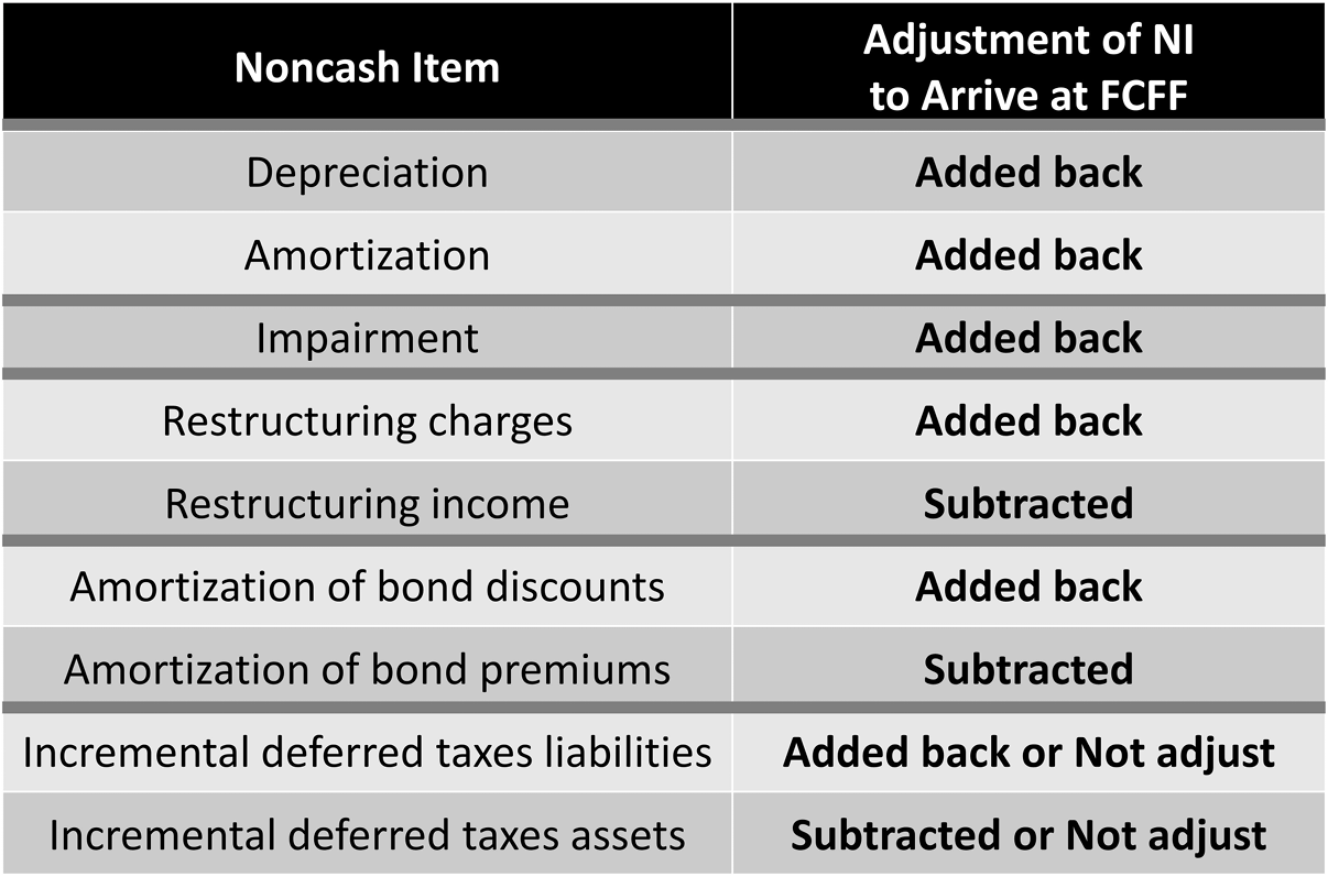
NCC is non-cash charges, which represent an adjustment for noncash decreases and increases in net income
FCInv is net fixed capital investment, which equals to capital expenditure less proceeds from sales
WCInv is working capital investment excluding cash and short-term debt (notes payable and current portion of long-term debt)
Expanding Formulas
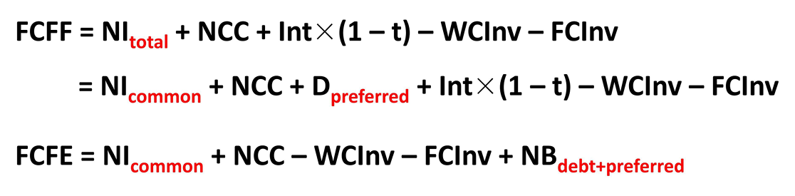
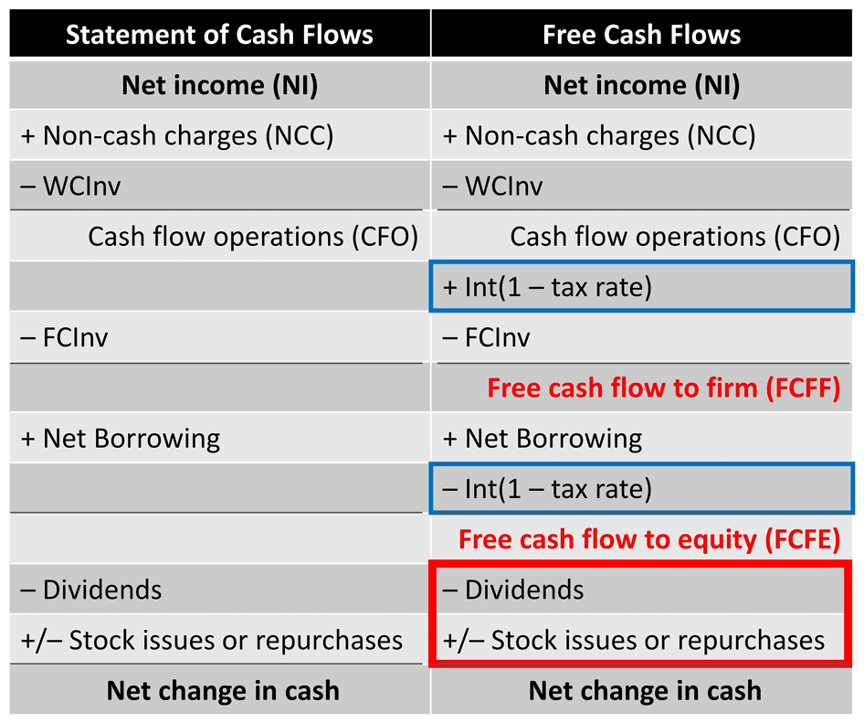
FCFF= NI+NCC+Int\times(1-t)-WCInv-FCInv
FCFF=EBITDA\times(1-t)+NCC\times t-WCInv-FCInv
FCFF=CFO+Int\times(1-t)-FCInv
Calculating FCFE
Basic Formula
FCFE=FCFF-Int \times(1-t)+NB
NB is net borrowings, which is debt issued less debt repaid over the period for which one is calculating free cash flow
NI is a Poor Proxy for FCFE
NI is a cash flow concept
NI recognizes non-cash charges such as depreciation, amortization
NI fails to recognize the cash flow impact of investments in working capital and net fixed assets, and net borrowings
EBITDA is a Poor Proxy for FCFE
EBITDA does not reflect taxes paid
EBlTDA ignores effect of depreciation tax shield
EBITDA does not account for needed investments in working capital and net fixed assets for going concern viability
EBlTDA is a pre-levered figure so it is pre-interest and before net borrowings
More Details About the Parameters
Non-Cash Charges
Working Capital Investments
Net investment in working capital for the purpose of calculating FCF excludes
Changes in cash and cash equivalents
Notes payable
Current portion of L.T.debt
There is an inverse (direct) relationship between changes in current assets (current liabilities) and changes in free cash flows
Fixed Capital Investments
Fixed capital investment (FCInv) represent a cash out flow necessary to support the company's current and future operations
Expenditures can include acquisition of intangible items such as trademarks
Care should be used with non-recurring large acquisitions in forecasts
Fixed capital investment is a net amount
It is equal to the difference between capital expenditures (investments in long-term fixed assets) and the proceeds from the sale of long-term assets
If there were no disposals of fixed assets
Given gross PP&E: FCInv= GV_{ending}-GV_{beginning}
Given net PP&E: FCInv = BV_{ending}- BV_{beginning} + \text{depreciation expense}
If there were disposals of fixed assets
Given gross PP&E: FCInv_{disposals}=FCInv +\text{AD of disposed assets}-\text{P/L from disposals}
Given net PP&E: FCInv_{disposals}=FCInv - \text{P/L from disposals}
Adjust FCFF if there were disposals of fixed assets
Calculate "FCInv = CAPEX - proceeds from disposal", Subtract P/L from disposals from NI
Net Borrowing
Net borrowings only affect FCFE, they do not affect FCFF
Notes payable
Increase in notes payable, add to FCFE
Decrease in notes payable, subtract from FCFE
Current portion of long-term debt
Increase in short-term debt, add to FCFE
Decrease in short-term debt, subtract from FCFE
Long-term debt
Add debt issuances to net income to arrive at FCFE
Subtract debt repurchases from net income to arrive at FCFE
Free Cash Flows with Preferred Stocks
For the most part, the discussion of FCFF and FCFE so far has assumed the company has a simple capital structure with two sources of capital, namely, debt and equity
Including preferred stock as a third source of capital requires the analyst to account for the dividends paid on preferred stock and for the issuance or repurchase of preferred shares
Usages of FCFs
Interesting Contrasts
Effects of Changing Leverage
An increase in leverage will not affect FCFF
Changing leverage (i.e. changing the amount of debt financing in the company's capital structure), does have some effects on FCFE particularly
An increase in leverage affects FCFE in two ways
In the year the debt is issued, it increases FCFE by the amount of debt issued
After the debt is issued, FCFE is then reduced by the after-tax interest expense
Estimations of FCFs
Approach one: forecast overall growth rate of FCFs
Calculate historical FCF
Estimate FCF for current period
Apply a constant growth rate to current FCF: FCF\times(1+g)^n
Usually, g_{FCFF}\ne g_{FCFE}
Approach two: forecast components of FCFs
Forecast each underlying component of FCFs
NI, NCC, FCInv and WCInv are tied to sales forecast
More realistic and flexible, but time consuming
Approach three: sales-based forecasting method
Investment in fixed capital in excess of depreciation (FCInv- Dep) and investment in working capital (WCInv) both bear a constant relationship to forecast increases in the size of the company as measured by increases in sales \frac{FCInv-Dep}{\Delta Sales} and \frac{WCInv}{\Delta Sales} will keep constant
Optimal capital structure represented by the debt ratio (DR) is constant DR=\frac{D}{D+E} will keep constant
Use FCFF when high or changing debt levels, negative FCFE
Single-stage, two or more stages?
Single-stage model for income stock(slow and constant growth)
More-stage models for whose competitive advantage will disappear over time
Total FCF or components of FCF?
Terminal value via GGM or Multiples?
Nominal or real?
International setting or volatile inflation rates: use real rates
Total value or value of the operating assets?
Free cash flow valuation focuses on the value of assets that generate operating cash flows
If a company has significant non-operating assets, such as excess cash, excess marketable securities, or land held for investment, then analysts often calculate the value of the firm as the value of its operating assets (as estimated by FCFF valuation) plus the value of its nonoperating assets
Sensitivity Analysis
Apply sensitivity to each of the following variables:
The base-year value for the FCFF or FCFE
Future growth rate
Risk factors: beta, risk free rate and ERP
Relationship between discount rate and the growth rate is critical In general
Most sensitive: Beta and growth rate of FCF
Less sensitive: r_f, and FCF.
Market-Based Valuation
Basic Concepts of Multiples
Introduction of Multiples
Price multiples are ratios of a stock's market price to some measure of fundamental value per share
The intuition is that investors evaluate the price of a stock by considering what a share buys in terms of per share earnings,net assets, cash flow, or some other measure of value
Enterprise value multiples relate the total market value of all sources of a company's capital to a measure of fundamental value for the entire company
Relative Valuation Method
The method of comparables (i.e. relative valuation method)involves using a multiple to evaluate whether an asset is relatively fairly valued, relatively undervalued, or relatively overvalued in relation to a benchmark value of the multiple
Choices for the benchmark include:
A closely matched individual stock
The average for peer group of companies or industry
Own history
The economic rationale for the methods of comparable is law of one price
Cross Border Valuation Differences
Comparing companies across borders frequently involves accounting method differences, cultural differences,economic differences, and resulting differences in risk and growth opportunities
For example, P/E ratios for individual companies in the same industry across borders have been found to vary widely
Justified Price Multiples
A justified price multiple (also called warranted price multiple or intrinsic price multiple) for the stock is the estimated fair value of multiples
Justified price multiples can be justified on the basis of 1) method of comparables or 2) method of forecasted fundamentals
Comparison
If actual price multiple = justified price multiple, then be properly valued
If actual price multiple < justified price multiple, then be undervalued
If actual price multiple > justified price multiple, then be overvalued
The method is based on forecasted fundamentals relates multiples to company fundamentals (growth, risk, payout) through DCF model, and may permit the analyst to explicitly examine how valuations differ across stocks and against a benchmark given different expectations for growth and risk
Price Multiples
PE ratio
Rationale and Drawbacks of PE ratio
Rationale for Using P/E Ratio
Earnings power is a chief driver of investment value
P/E ratio is widely recognized and used by investors
Differences in stock's P/Es may be related to differences in long-run average returns on investments in those stocks, according to empirical research
Potential Drawbacks of P/E Ratio
Negative and very low earnings make P/E useless
Volatile or transitory earnings make interpretation difficult
Management discretion on accounting choices can distort earnings
Solely using the ratio avoids addressing the fundamentals (growth, risk, and cash flows)
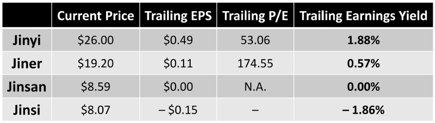
Trailing and Leading P/E Ratio
Trailing P/E_0 (a.k.a. current P/E), is stock's current market price divided by the last four quarters (or past 12 months) EPS
In such calculations, EPS is sometimes referred to as "trailing 12 month (TTM) EPS"
Leading P/E_1 (a.k.a. forward P/E or prospective P/E), is stock's current market price divided by next year's expected EPS
Analysts interpreted "next year's expected earnings" as expected EPS for:
next four quarters
next 12 months (NTM P/E)
next fiscal year
Problems with Trailing P/E Ratio
Transitory and non-recurring components of earnings are company-specific
Non-recurring earnings are needed to be removed because valuation focus on future cash flows, so we calculate underlying earnings (persistent earnings, continuing earnings, or core earnings)
Non-recurring items to remove include: Gains/losses on asset sales; Asset write-downs for impairment; Loss provisions; Changes in accounting estimates
Cyclicality components of earnings due to business or industry trends
The countercyclical property of P/E (Molodovsky Effect)
Analysts should calculate normalized EPS to remove cyclical component of earnings and capture mid-cycle earnings under normal market conditions
Differences in accounting methods
Potentialdilution of EPS
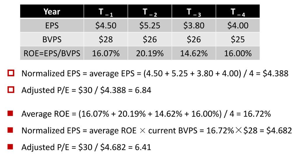
Normalized Earnings
Method 1: historical average EPS
Normalized EPS is the average EPS over the most recent full cycle
Method 2: average ROE
Normalized EPS is the average ROE from the most recent full cycle multiplied by current book value per share
Method 2 is preferred since it more accurately reflects the effect of growth in company size on EPS
Example
Justified P/E Ratio
Fundamental factors affecting justified P/E ratio
Justified P/E positively related to growth rate and payout ratio, "all else equal"
Justified P/E inversely related to required return (real rate, inflation and equity risk premium), "all else equal"
Terminal Value Estimation
Terminal value is the intrinsic value projected at end of estimation horizon
Using fundamentals: Requires estimates of g, r, and payout
Using comparables: Uses market data to calculate benchmark
Predicted P/E from Regression
The P/E ratios may be regressed against the stock and company characteristics
The estimated equation exhibits the relationship between P/E and stock's characteristics
Positive coefficient with growth rate and payout ratio
Negative coefficient with beta
Limitations of regression
The method captures valuation relationships only for the sample of stock over a particular time period, and the predictive power of the regression for a different stock and different time period is not know
The relationship between P/E and fundamentals may change over time
Multicollinearity(correlation within linear combinations of the independent variables)
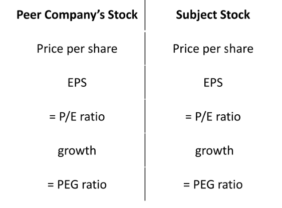
P/E-to-Growth[PEG] Ratio
PEG ratio is calculated as the stock's P/E divided by the expected earnings growth rate (in percentage terms)
PEG ratio is a calculation of a stock's P/E per percentage point of expected growth
Stocks with lower PEGs are more attractive than stocks with higher PEGs, all else being equal
PEG is useful but must be used with care for several reasons
PEG assumes a linear relationship between P/E and growth rate
The model for P/E in terms of the DDM shows that, in theory, the relationship is not linear
PEG does not factor in differences in risk, an important determinant of P/E
= PEG does not account for differences in the duration of growth
For example, dividing P/Es by short-term growth forecasts may not capture differences in long-term growth prospects
Valuation Based on Comparables
Peer company multiples
The subject stock's P/E is compared with the median or mean P/E for the peer group to arrive at a relative valuation
Are observed differences between P/E ratios explained by underlying determinants of P/E?
If not, asset may be mispriced
Industry and sector multiples
Using industry and sector data can help an analyst explore whether the peer-group comparison assets are themselves appropriately priced
Own historical P/E
Analyst shall be alert to the impact on P/E levels of changes in a company's business mix and leverage overtime
Changes in the interest rate environment and economic fundamentals over different time period can be another limitations
Overall Market Multiples
The question of whether the overall market is fairly priced has captured analyst interest throughout the entire history of investing
Fed Model
The stock market is to be overvalued when the stock market's current earnings yield is less than the 10-year Treasury bond (T-bond) yield
Fed Model uses expected earnings for the next 12 months in calculating the ratio
Yardeni Model
Yardeni obtained the following expression for the justified P/E on the market
\frac{P}{E}=\frac{1}{C B Y-b \times L T E G}
CBY is current Moody's Investors Service A-rated corporate bond yield LTEG is the consensus five-year earnings growth rate forecast for market index b measures the weight the market gives to five-year earnings projections
Higher current corporate bond yield imply a lower justified P/E
Higher expected long-term growth results in a higher justified P/E
Earnings Yield and Dividend Yield
Ranking Stocks by P/E Ratio
Stock selection disciplines that use P/E ratios often involve ranking stocks
The security with the lowest positive P/E has the lowest purchase cost per currency unit of earnings among the securities ranked
Zero earnings and negative earnings pose a problem if the analyst wishes to use P/E as the valuation metric
Because division by zero is undefined, P/Es cannot be calculated for zero earnings
A "negative P/E security" will rank below the lowest positive P/E security, but the negative earning security is actually the most costly in terms of earnings purchased
Earnings Yield
If the analyst is interested in a ranking, however, one solution is the use of reciprocal of the original ratio, which places"price" in the denominator
In the case of the P/E, the inverse price ratio is earnings yield
Ranked by earnings yield from highest to lowest, the securities are correctly ranked from cheapest to most costly
In addition to zero and negative earnings, extremely low earnings can pose problems when using P/Es, particularly for evaluating the distribution of P/Es of a group of stocks under review. In this case, inverse price ratios can be useful
An extremely high P/E (an outlier P/E) can overwhelm the effect of the other P/Es in the calculation of the mean P/E
Although the use of median P/Es and other techniques can mitigate the problem of skewness caused by outliers, the distribution of inverse price ratios (earnings yield) is inherently less susceptible to outlier-induced skewness
Dividend Yield
Rationales for using dividend yield(D/P)
Dividend yield is a component of total return
Dividends are a less risky component of total return than capital appreciation
Drawbacks for using dividend yield(D/P)
Dividend yield is just one component of total return
Dividends paid now displace earnings in all future periods (dividend displacement of earnings)
Trailing dividend yield and Leading dividend yield
Trailing dividend yield is the dividend rate (annualized amount of the most recent dividend) divided by the current market price
Leading dividend yield is the forecasted dividends over the next year divided by the current market price
Justified Dividend Yield
Justified leading dividend yield
\frac{D_1}{V_0}=\frac{D_1}{\frac{D_1}{r-g}}=r-g
An analyst can generally use P/B when EPS is zero or negative
BVPS is usually positive
P/B maybe more meaningful than P/E when EPS is abnormally high or low or is highly variable
Book value of equity is more stable than EPS
BVPS has been viewed as appropriate for valuing companies composed chiefly of liquid assets, such as finance, investment,insurance, and banking institutions
Book value has also been used in the valuation of companies that are not expected to continue as a going concern
Potential Drawbacks for Using P/B Ratio
Does not reflect value of intangible assets, off-B/S assets(e.g., human capital)
Misleading when comparing firms with significant differences in asset size
Different accounting conventions obscure comparability (particularly international)
Inflation and technological change can cause big differences between BV and MV
Share repurchase and issuances may distort historical comparison
Adjustments to P/B Ratio
To make the book value more accurately reflect the value of shareholders' investment or to make P/B more comparable among different stocks
May calculate tangible book value per share
Certain adjustments may be appropriate for enhancing comparability
For example, restate the book value of the company using LIFO
The balance sheet should be adjusted for significant off-balance items
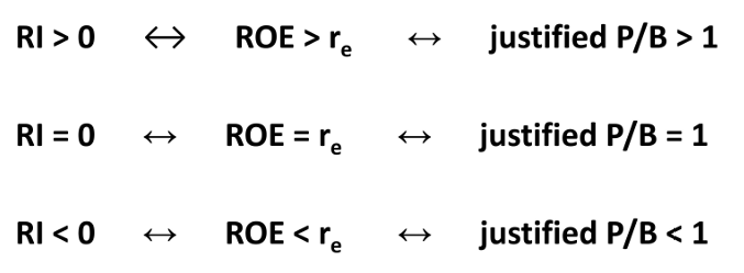
Justified P/B Ratio
Formula
\begin{aligned} \text { Justified P/B ratio } & =\frac{V_0}{B V\left(E_0\right)}=\frac{\frac{D_1}{r-g}}{B V\left(E_0\right)}=\frac{\frac{D_1}{B V\left(E_0\right)}}{r-g}=\frac{\frac{N I_1\times(1-b)}{B V\left(E_0\right)}}{r-g} \\ & =\frac{R O E \times(1-b)}{r-g}=\frac{R O E-R O E \times b}{r-g}=\frac{R O E-g}{r-g}\end{aligned}
Fundamental factor affecting P/B ratio
Spread between ROE and r increases → value creation → higher market value
P/B increases as ROE increases
P/B increases as g increases
P/B increases as r decreases
(falling risk, interest rates, inflation and beta)
P/S Ratio
Rationales for Using P/S Ratio
P/S is useful for distressed firms
Sales revenue is often positive
Sales are generally more stable and less prone to distortion than EPS over time
P/S is useful for mature, cyclical, and zero-income stocks
Differences in P/S ratios may be related to difference in long-run average returns
Potential Drawbacks for Using P/S Ratio
High sales growth does not translate to operating profitability
P/S ratio does not capture different cost structures between firms
Revenue recognition methods can distort reported sales and forecasts
Adjusted CFO
Adjustments to CFO for components not expected to persist into future time periods
Adjustments to CFO may be required when comparing companies that use different accounting standards.
EBITDA
FCFE may be a cash flow concept with the strongest link to valuation theory
Rationales for Using P/CF Ratio
It is more difficult to manipulate CF than EPS
Cash flow is more stable than earnings
Addresses quality of earnings problem
Differences in P/CFs may explain differences in long-run average returns
Potential Drawbacks for Using P/CF Ratio
Earnings plus non-cash charges approach ignores some cash flows such as net fixed investments, working capital investment and net borrowings
FCFE is preferable to CFO, but FCFE more volatile and more difficult to compute, and can be negative with large CapEx
Some companies have increased their use of accounting methods that enhances cash flow measures
Operating cash flows under IFRS may not be comparable to operating cash flow under US GAAP
Enterprise Value Multiples
Enterprise value to EBITDA
Enterprise value multiple provides an indication of company/firm value, not equity value
Enterprise value to EBITDA (EV/EBITDA) is by far the most widely used enterprise value multiple
Because the numerator is enterprise value, EV/EBITDA is a valuation indicator for the overall company rather than common stock
EBITDA is a earnings flow to both debt and equity holders
Rationales for using EV/EBITDA ratio
Appropriate for comparing firms with different financial leverage since EBITDA is pre-interest
Controls for depreciation/amortization differences among businesses
EBITDA usually positive when EPS is negative
Potential drawbacks for using EV/EBITDA ratio
lgnores changes in working capital investments
FCFF (which controls for capital expenditures) is more closely tied to value
Enterprise Value
Enterprise Value(EV) = MV of common stock + MV of preferred stock + MV of debt - cash and cash equivalents - short-term investments
Cash and investment are subtracted because EV is designed to measure the net price an acquirer would pay for the company
Total invested capital(TIC) (a.k.a. market value of invested capital) is an another measure of total firm value, that is an alternative to enterprise value
Total invested capital(TIC) = MVof common stock + MVof preferred stock + MV of debt
Valuation Based on Forecasted Fundamentals
As with other multiples, intuition about the fundamental drivers of enterprise value to EBITDA can help when applying the method of comparables
All else being equal, the justified EV/EBITDA based on fundamentals should be
Positively related to the expected growth rate in free cash flow to the firm
Negatively related to the business's weighted average cost of capital
Positively related to expected profitability as measured by return on invested capital
ROIC is the relevant measure of profitability because EBITDA flows to all providers of capital
Other Enterprise Value Multiples
EV/FCFF
EV/EBITDAR(where R stands for rent expense)
It is favored by airline industry analysts
Enterprise value-to-sales(EV/S)
Price-to-sales ratio has the conceptual weakness that some of the proceeds from the company's sales will be used to pay interest and principal to the providers of the company's debt capital
A P/S for a company with little or no debt would not be comparable to a P/S for a company that is largely financed with debt, however EV/S would be the basis for a valid comparison in such a case
Momentum valuation indicators
Momentum Valuation Indicators
Momentum indicators are the valuation indicators that relate either price or a fundamental to the time series of their own past values
Momentum investment strategies
Buy winners, sell losers
Contrary investment strategies
Buy losers, sell winners
Unexpected Earnings
Unexpected earnings (also referred to as earnings surprise) is the difference between reported EPS and expected EPS
\mathrm{U E}_\mathrm{t}=\mathrm{E P S}_\mathrm{t}-\mathrm{E}\left(\mathrm{E P S}_\mathrm{t}\right)
The rationale is that positive surprise may be associated with persistent positive abnormal return,or alpha
Another momentum indicator based on the relative change in earnings per share is called standardized unexpected earnings
\mathrm{SUE}_{\mathrm{t}}=\frac{\mathrm{EPS}_{\mathrm{t}}-\mathrm{E}\left(\mathrm{EPS}_{\mathrm{t}}\right)}{\sigma_{\left[\mathrm{EPS}_{\mathrm{t}}-\mathrm{E}\left(\mathrm{EPS}_{\mathrm{t}}\right)\right]}}
Relative Strength Indicators
Relative strength indicators compare a stock's performance during a period 1) to its own past performance or 2) to the performance of some group of stocks
The simplest relative strength indicator of the first type is the stock's compound rate of return over some specified time
A simple relative strength indicator of the second type is the stock's performance divided by the performance of an equity index
This indicator maybe scaled to one at the beginning of the study period and if the stock goes up quickly (slowly) than the index, then relative strength will be above (below) one
Central tendency
Measuring Central Tendency in Multiples
Arithmetic mean
Most affected by outliers
Median
Least affected by outliers
Harmonic mean
Less affected by large outliers, more affected by small outliers
Weighted harmonic mean
Effect of outliers depend on market value weight
Harmonic mean
X_H=\frac{n}{\sum_{i=1}^n \frac{1}{X_i}}
Less weight on higher ratios
Reduces impact of large outliers
More weight on lower ratios
The harmonic mean may aggravate the impact of small outliers,but such outliers are bounded by zero on the downside
Lower value than arithmetic mean
Unless all observations are the same value
Used when market weight information unavailable
Weighted Harmonic Mean
X_{WH}=\frac{n}{\sum_{i=1}^n \frac{w_i}{X_i}}
Similar to simple harmonic mean except in weighting
Uses market value weights
Corresponds to portfolio value and can reflect the true "average P/E"(e.g., total price/total earnings)
Residual Income Valuation
Concepts of Residua Income
Introduction of Residual Income
Residual income (RI) is net income less a charge (deduction) for shareholders' opportunity cost
Residual income explicitly deducts all capital costs of both debt and equity, so it is the "residual or remaining income" after considering the costs of all of a company's capital
Residual income has sometimes been called "economic profit"
The cost of equity(r_e) is the marginal cost of equity, because it represents the cost of additional equity
It is also referred to as the required rate of return on equity
Introduction of Residual Income Models
The appeal of residual income models stems from a shortcoming of traditional accounting
A company that is generating more income than its cost of obtaining capital (that is, one with positive residual income) is creating value
In forecasting future residual income, the term "abnormal earnings" is also used
In the long term, companies that earn more (less) than the cost of capital should sell for more (less) than book value
Formula to Calculate RI
Basic Formula
R I_t=N I_t-B V\left(E_{t-1}\right) \times r_e
R I_t=B V\left(E_{t-1}\right) \times\left(R O E_t-r_e\right)
Alternative Formula
\mathrm{RI}_{\mathrm{t}} =\text { NOPAT }_{\mathrm{t}}-\text { total capital charge }_{\mathrm{t}} =\text { EBIT }_{\mathrm{t}} \times(1-\text { tax rate })-\left(\text { cost of debt capital }_{\mathrm{t}}+\text { cost of equity capital }_{\mathrm{t}}\right)
Violations of clean surplus relationship occur when items bypass the income statement and direct adjustments to equity are made
Examples for considerations
Unrealized changes in the fair value of some financial instruments
Foreign currency translation adjustments
Certain pension adjustments
Portion of gains and losses on certain hedging instruments
Changes in revaluation surplus related to property, plant, and equipment or intangible assets (applicable under IFRS but not under US GAAP)
For certain categories of liabilities, change in fair value attributable to changes in the liability's credit risk(applicable under IFRS but not under US GAAP)
Balance Sheet Adjustments for Fair Value
To have a reliable measure of book value of equity, an analyst should identify and scrutinize significant off-balance-sheet assets and liabilities
Additionally, reported assets and liabilities should be adjusted to fair value when possible
Examples for considerations
Inventory
Deferred tax assets and liabilities
Operating leases
Reserves and allowances
Intangible Items
Intangible items require special consideration because they are often not recognized as an asset unless they are obtained in an acquisition
For example, advertising expenditures can create a highly valuable brand, but they are shown as an expense, and the value of a brand would not appear as an asset on the financial statements unless the company owning the brand was acquired
Research and development(R&D) costs provide another example of an intangible asset that must be given careful consideration
If a company engages in unproductive R&D expenditures, these will lower residual income through the expenditures made
If a company engages in productive R&D expenditures, these should result in higher revenues to offset the expenditures over time
Nonrecurring Items
Companies often report nonrecurring charges as part of earnings, which can lead to overestimates and underestimates of future residual earnings if no adjustments are made
Example for considerations
Unusual items
Extraordinary items
Restructuring charges
Discontinued
Accounting changes
Other Aggressive Accounting Practices
Companies may engage in accounting practices that result in the overstatement of assets (book value) and/or overstatement of earnings
Other activities that a company may engage in include accelerating revenues to the current period or deferring expenses to a later period
Conversely, companies have also been criticized for the use of "cookie jar" reserves (reserves saved for future use), in which excess losses or expenses are recorded in an earlier period
Accounting Issues-International Considerations
Accounting standards differ internationally and these differences result in different measures of book value and earnings internationally
It suggests that valuation models based on accrual accounting data might not perform as well as other valuation models in international contexts
Commercial implementations
Economic Value Added
Economic value added(EVA) = NOPAT - (C% × TC)
NOPAT is the company's net operating profit after taxes
C% is the cost of capital
TC is total capital
In EVA model, both NOPAT and TC are adjusted for a number of items
Because of the adjustments made in calculating EVA, a different numerical result may be obtained, in general, than that resulting from the use of the simple computation of RI (economic profits)
Economic value added (EVA) measures valued added to shareholders by management
Some of the more common adjustments include the following
Research and development (R&D) expenses are capitalized and amortized rather than expensed
Deferred taxes are eliminated such that only cash taxes are treated as an expense
Any inventory LIFO reserve is added back to capital, and any increase in the LIFO reserve is added in when calculating NOPAT
Operating leases are treated as capital leases, and nonrecurring items are adjusted
Market Value Added
Market value added (MVA) = market value of the company - accounting book value of total capital
A company that generates positive economic profit should have a market value in excess of the accounting book value of its capital
Analysts should evaluate the change in MVA over time
MVA measures the effect on value of management's decisions since the firm's inception
Tobin's Q
Tobin's q = Market value of debt and equity / Replacement cost of total asssets
Denominator uses assets that are valued at replacement cost rather than at historical accounting cost
Replacement costs take into account the effects of inflation
Valuation Models
Single-Stage Residual Income Model
If we assume constant growth rate for residual income
V_0=B_0+\sum_{i=1}^{+\infty} \frac{R_i}{\left(1+r_e\right)^i}=B_0+\frac{R_1}{r_e-g}=B_0+\frac{B_0\times\left(R O E-r_e\right)}{r_e-g}=B_0\times \frac{R O E-g}{r_e-g}
\frac{RI_1}{r_e-g} is the additional value generated by the firm's ability to produce returns in excess of the cost of equity, and consequently, it is the present value of a firm's expected economic profits
In practice, if we use single-stage residual income valuation model,we always assume that a company has a constant return on equity and constant earnings growth rate through time
Multi-Stage Models-Using P/B Ratio
The main task here is to solve the PV of continuing residual income
V = B + PV(interim high-growthRI) + PV(continuing RI)
One finite-horizon model of residual income valuation assumes that at the end of time horizon T, a certain premium over book value P^\ast_T-B_T exists for the company
V_0=B_0+\sum_{t=1}^T \frac{N_t-r \times B_{t-1}}{(1+r)^t}+\frac{P_T^*-B_T}{(1+r)^T}
The essence here is that the Rl will decline to mature industry level
The longer the forecast period, the greater the chance the company's residual income will converge to zero, thus P^\ast_T-B_T may be treated as zero
Continuing Residual Income
Situation I: RI will drop immediately to zero after year T
PV_T=0
PV_0=0
Situation II: RI will persist at current level forever
PV_T=\frac{RI_{T+1}}{r_e}=\frac{RI_{T}}{r_e}
PV_0=\frac{PV_T}{(1+r_e)^T}
Situation III: RI will decline over time to zero after year T
PV_T=\frac{RI_{T+1}}{1+r_e-\omega} \omega is a persistence factor, which is between zero and one
PV_0=\frac{PV_T}{(1+r_e)^T}
Situation IV: RI will decline to mature industry level at the end of year T
PV_T=P_T^\ast-B_T=(P/B)_t\times B_T-B_T
PV_0=\frac{PV_T}{(1+r_e)^T}
Persistence Factor
Factors suggesting higher\omega
Low dividend payout
Strong market leadership positions
High historical persistence in the industry
Factors suggesting lower\omega
Extreme accounting rates of return(ROE)
Extreme levels of special items
Extreme levels of accounting accruals
Model Comparisons
DDM
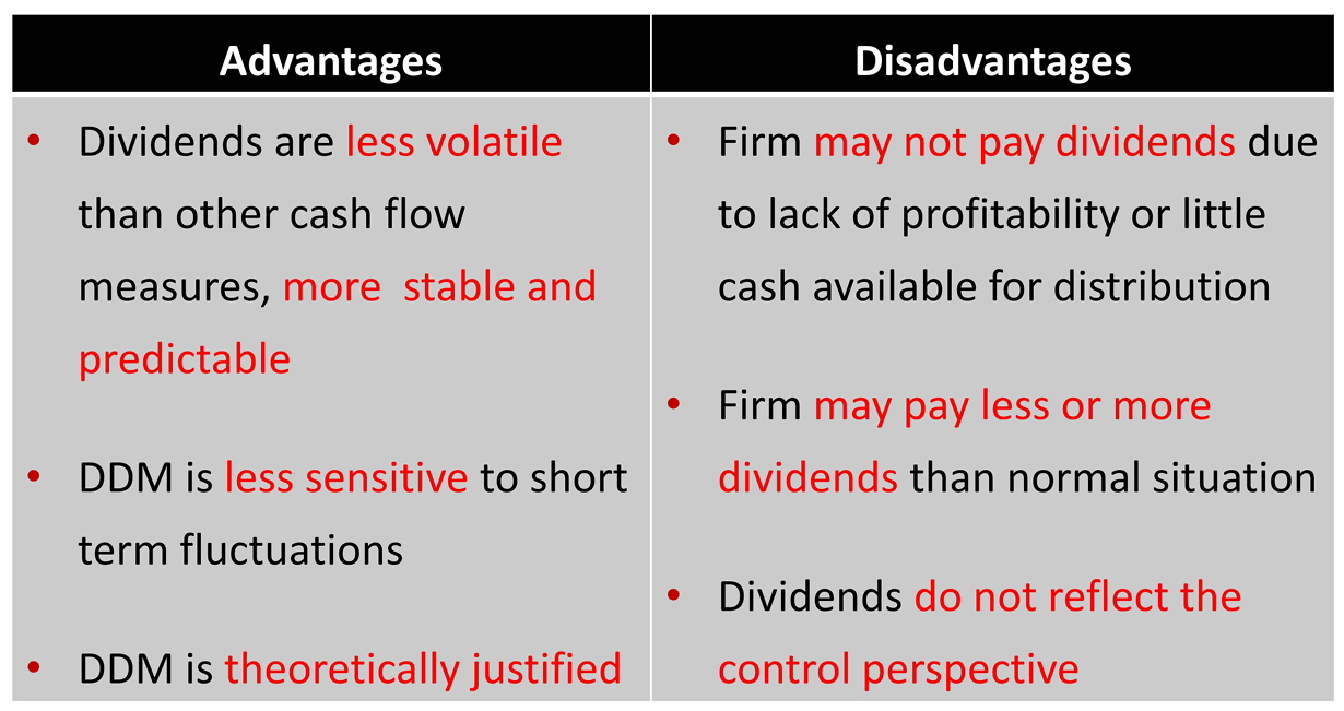
Advantages of DDM
Investors generally receives cash returns only in the form of dividends
The relative stability of dividends may make DDM values less sensitive to short-run fluctuations in underlying value than alternative DCF models
Analysts often view DDM values as reflecting long-run intrinsic value
Disadvantages of DDM
A company might not pay dividends on its stock
Predicting the timing of dividend initiation and the magnitude of future dividends without any prior dividend data is generally not practical
Dividends may not reflect the control perspective desired by the investor
Appropriateness for using DDM
The company is dividend-paying (i.e., the analyst has a dividend record to analyze)
The board of directors has established a dividend policy that bears an understandable and consistent relationship to the company's profitability
The investor takes an on-control perspective Mature firms, profitable but not fast growth
FCF Model
Advantages of FCF model
Popular in current investment practice
The record of free cash flows can also be examined even for a non-dividend-paying company
FCFE can be viewed as measuring a company's capacity to pay dividends
Disadvantages of FCF model
Negative free cash flow, resulting from large capital expenditure demands
May require long forecast periods for CF to turn positive, introducing greater model uncertainty
Appropriateness for using FCF model
No dividend payment history
Dividends not related to earnings or dividends and FCF differ significantly
FCF consistent with profitability within a reasonable time period
Controlling shareholder perspective
RI Model
Advantages of RI model
Wide applicability, even if FCF < 0
Used for dividend and non-dividend paying firms
Incorporates opportunity cost of capital for both debt and equity holders
Brings recognition value closer to the present by focusing on current book value plus forecasted residual income
Disadvantages of RI model
Application of the RI model requires a detailed knowledge of accrual accounting
The quality of accounting disclosure can make the use of Rl valuation less robust and more error prone
RI model is appropriate when
No dividends or volatile dividends
Negative free cash flows
Uncertainty in forecasting terminal values
RI model is not appropriate when
Clean surplus solution violated significantly
Unreliable estimates of BV and ROE
Private Company Valuation
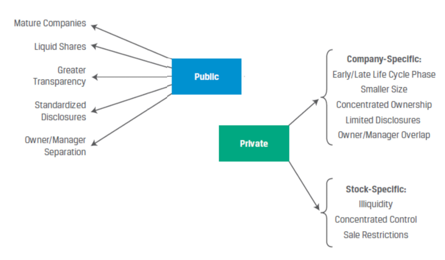
Public vs.Private Company Valuation
Public Versus Private Company Features
The valuation of smaller firms often warrants the use of a higher required rate of return due to greater income variability and risk resulting from:
fewer and less-diversified lines of business and customers;
less well developed marketing, sales, and distribution;
limited growth prospects because of reduced access to capital.
Company-specific factors may be positive or negative.
The senior management of many private firms often has a controlling ownership interest. This feature greatly reduces the principal-agent problem which may arise when owners and managers are separate.
Private equity firms often acquire underperforming public companies to restructure, divest, or acquire lines of business while under private ownership and control with the goal of selling the reorganized firm at a higher price to another private buyer or the public via an IPO
Private company managers can take a longer-term perspective in strategic decision making without pressure from external investors seeking short-term gains on publicly traded shares.
Family Ownership of Private Companies
Family owned and operated businesses dominate the private company landscape in many developed and developing economies.
The small and medium-sized enterprises in the German-speaking countries of Germany, Austria, and Switzerland known as the Mittelstand are predominantly family owned and managed.
Private company valuation often plays an important role as business owners consider turning over control to non-family managers while retaining ownership, accessing external capital, or selling a minority stake or the entire business.
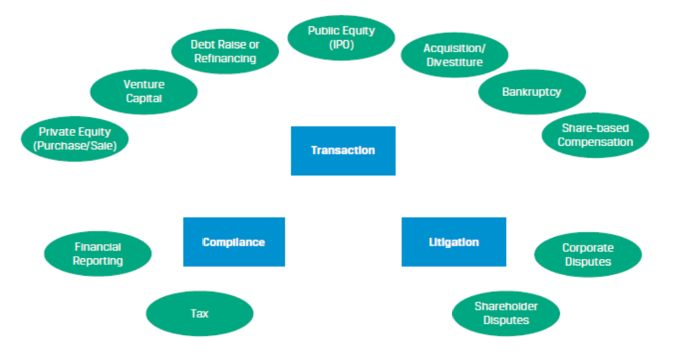
Private Company Valuation Uses and Areas of Focus
Transaction-related valuations(transfer of ownership or incremental financing)
Venture capital financing (early stage); Private equity financing (growth or buyout stage);Debt financing; Initial public offering (IPO); Acquisitions and divestitures; Bankruptcy; Share-based incentive compensation
Compliance-related valuations(compliance and litigation purposes)
Financial reporting; Tax reporting; Litigation
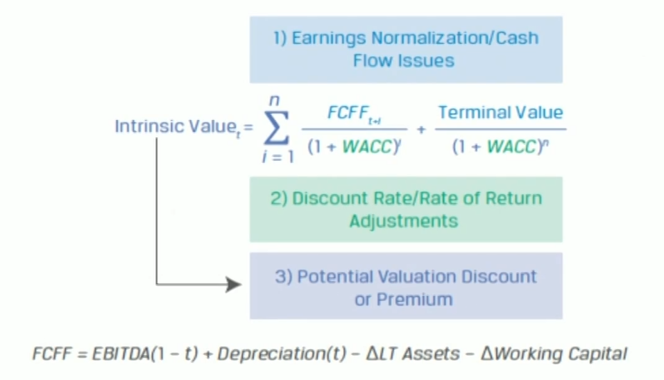
Three key areas related to private company valuation warrant the particular attention of analysts
Cash Flow and Earnings Adjustments: analysts must first identify and adjust key balance sheet and income statement items to address private versus public company differences to estimate a company's normalized earnings.
Discount Rate and Rate of Return Adjustments: due to the lack of observable market prices for debt and equity, the assumptions associated with the CAPM for public companies often do not apply to private companies and require estimation and adjustment
Valuation Discount or Premium: stock-specific considerations related to either the benefit of greater control or the drawback of illiquidity and a minority interest in a business with lesser control must be factored into a company's valuation.
Areas of Focus on Private Company Valuation
Earnings Normalization Issues for Private Companies
Private companies may have their financial statements reviewed rather than audited.
Reviewed financial statements involve an opinion letter with representations and limited assurances by the reviewing accountant and a less thorough review than for audited financials
Compiled financial statements are the most basic approach and are unaccompanied by an auditor's opinion letter.
Reviewed or compiled statements usually require adjustment.
Earnings Normalization and Cash Flow Estimation
Normalized earnings
Private company valuation: specific adjustments for non-recurring,non-economic items as well as for ongoing anomalies which prevent direct comparisons to publicly owned entities.
Related Party Transaction: A related party transaction is one between parties which share economic or other interests
An arm's length transaction is one between independent parties acting in their own self-interest which occur and are recorded at or near fair market value.
Cash Flow Estimation Issues for Private Companies
Specific challenges associated with private company cash flow valuation include the nature of the interest being valued,potentially acute uncertainties regarding future operations, and managerial involvement in forecasting.
A valuation based upon scenario analysis is a common approach.
Factors Affecting Private Company Discount Rates
Application of size premiums to discount rates.
Relative debt availability and cost of debt.
Private company may have less access to debt financing than similar public company. Reduced debt access may lead a private company to rely more on equity financing,which would tend to increase its WACC
A smaller private company could face greater operating risk and a higher cost of debt
Discount rates in an acquisition context.
When larger, more mature companies acquire smaller, riskier target companies, the buyer would be expected to have a lower cost of capital than the target.
Discount rate adjustment for projection risk would typically be highly judgmental.
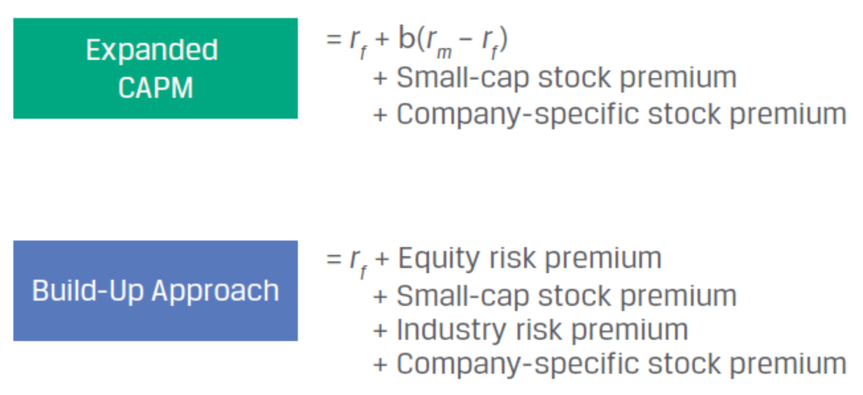
Required Rate of Return Models
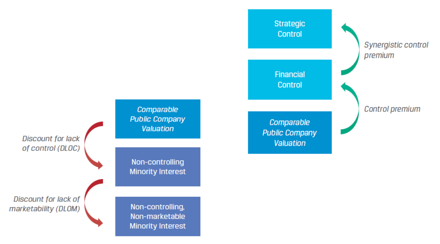
Valuation Discounts and Premiums
Strategic buyer: this value reflects a buyer who intends to use their controlling stake to take action to increase firm revenue and/or decrease costs beyond current expectations in order to increase the company's value.
Financial buyer: may be willing to pay a premium for a controlling interest for a private firm but is either unable to identify any synergies from a controlling interest, may be unable or unwilling to take advantage of them due to a lack of operational or management expertise, or has limited risk appetite.
Discount for lack of control (DLOC): involves a deduction from the pro rata share of 100% of the value of an equity interest to reflect the absence of some or all powers of control.
A lack of control may be disadvantageous to an investor because of the inability to select directors, officers, and management that control an entity's operations.
DLOC= 1- [1 / (1 + Control premium)]
Discount for lack of marketability (DLOM): is a deduction from an ownership interest's value to reflect the relative absence of a liquid market for a company's shares.
Develop marketability discount estimates. Restricted stock: The sale of blocks of restricted stock that exceed public trading activity in the stock.
The relationship of stock sales prior to IPOs: early-stage or high-growth companies approaching an IPO, an increase in value may result from lower risk and uncertainty as a company progresses in its development.
Option-based approaches: an at-the-money put option is priced; The put option premium as a percentage of the stock value provides an estimate of the DLOM.
Total Discount = [1 - (1 - DLOC) × (1 - DLOM)]
Private Company Valuation Approaches
Approaches for Private Company Valuation
The income approach values an asset as the present discounted value of the income expected from it
The market approach values an asset based on pricing multiples from sales of assets viewed as similar to the subject asset
The asset-based approach values a private company based on the values of the underlying assets of the entity less the value of any related liabilities
Income Approach
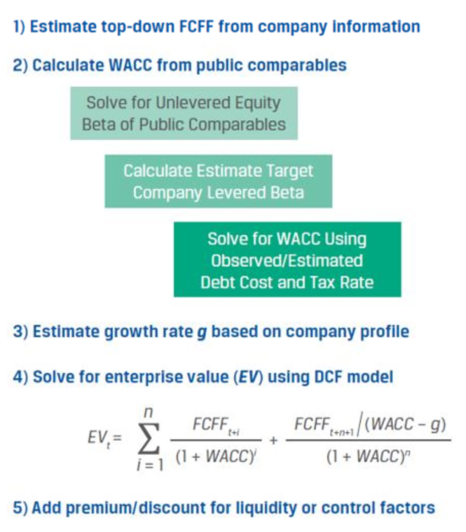
Free cash flow method
Capitalized cash flow method
CCM estimates value based on a company's projected performance as a growing perpetuity under the assumption of stable growth.
\text{Firm Value}_t=\frac{F C F F_{t+1}}{W A C C-g}
The expected FCFF may be estimated using the company's expected after-tax EBIT and the firm's reinvestment rate
\begin{align}
&\text { Firm Value }_t=\frac{\text { EBIT }_{t+1}(1-t)(1-\text { RIR })}{\text { WACC }-g}
\\
&\text { Revinvestment rate }=\mathrm{RIR}=\frac{g}{\mathrm{WACC}}
\end{align}
To solve for the intrinsic equity value, we must subtract the estimated market value of debt from firm value.
A constant WAcC---the capital structure will remain unchanged.
Estimate the market value of private debt when traded market values are unavailable.
Debt represents a small fraction --the face value of debt
Significant leverage, changing financial conditions, significant volatility--significant premium or discount from face value
FCFE excludes payments to debtholders and uses the cost of equity.
The denominator is referred to as the capitalization rate.
I V_t=\frac{\mathrm{FCFE}_{t+1}}{r_e-g}
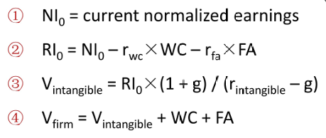
Excess earnings method
Market-Based Approach
Guideline Public Company Method(GPCM)
The PE ratio are frequently cited in the valuation of public companies, while metrics such as EV are more common in private company valuation as they offer greater flexibility to accommodate changes to the capital structure over the valuation period.
It is important to consider not only firms from the same industry but also firms of similar size, leverage, and stage in the company life cycle when choosing comparable.
Control premiums may be used in valuing a controlling interest in a company.
Several factors require careful consideration in estimating a control premium.
Type of transaction: strategic buyer > financial transactions
Industry factors: different time reflect different environment
Form of consideration: the exchange of stock or cash
Advantage of GPCM: potentially large pool of guideline companies and significant financial and trading information available
Disadvantage of GPCM: issues regarding to comparability and subjectivity in the risk and growth adjustment
Guideline Transactions Method (GTM)
Guideline Transactions(GTM) uses pricing multiples derived from acquisitions of public or private companies.
Transaction multiples would be the most relevant evidence for valuation of a controlling interest in a private company.
Several factors must be considered in assessing transaction-based pricing multiples:
Synergies
Contingent consideration
Non-cash consideration
Availability of transactions
Changes between transaction date and valuation date
Prior Transaction Method(PTM)
The prior transaction method (PTM) uses the actual price paid for shares or the price multiples implied by past transactions in the stock of the subject private company as the guideline
PTM is most relevant when considering the value of a minority equity interest in a company
Disadvantage of PTM: Historical transactions in the subject stock are very limited
Asset-Based Approach
The value of equity is calculated as the fair value of total assets less the fair value of total liabilities
Appropriateness
Not used for going concerns
Usually the lowest valuation
Difficulties in valuation:
Individual assets, Specialized assets, Intangibles